``[Dynamic] also has a very interesting property as an adjective, and that is it’s impossible to use the word, dynamic, in a pejorative sense. Try thinking of some combination that will possibly give it a pejorative meaning. It’s impossible. Thus, I thought dynamic programming was a good name.’’ - Richard Bellman

Example: Consumption & Savings

\[ \max_{\{c_t\}_{t=0}^\infty,\{s_t\}_{t=1}^\infty} \sum_{t=0}^\infty \beta^t u(c_t) \text{ s.t. } s_{t+1} = (1+r_t)(s_t - c_t) \]

Finite Horizon

\[ \max_{c_T} u(c_T) \text{ s.t. } s_{T+1} = (1+r_T)(s_T -c_T) = 0 \]

• Value function defined recursively \(V_T(s) = u(s)\) \[ \begin{aligned} V_{t-1}(s) = \max_{c_{t-1},s'} & u(c_{t-1}) + \beta V_{t}(s') \\ \text{ s.t.} & s' = (1+r_{t-1})(c_{t-1}-s) \end{aligned} \]
• Bellman equation

``An optimal policy has the property that whatever the initial state and initial decision are, the remaining decisions must constitute an optimal policy with regard to the state resulting from the first decision.’’ (Bellman 1962)

Example: Consumption & Savings

\[ \begin{aligned} \max_{\{c_t\}_{t=0}^\infty,\{s_t\}_{t=1}^\infty} & \sum_{t=0}^\infty \beta^t u(c_t) \\ \text{ s.t. } & s_{t+1} = (1+r)(s_t - c_t) \end{aligned} \]

• Starting with \(t=0\) or \(t=1\) or \(t=s\) gives same maximization
• Value function should not depend on time

\[ V(s) = \max_{c,s'} u(c) + \beta V(s') \text{ s.t. } s' = (1+r)(s-c) \] - How do we know that \(V\) exists? unique?

General Setup

\[ \begin{aligned} \max_{c_t,s_t} & \sum_{t=0}^\infty \beta^t u(c_t,s_t) \\ \text{s.t.} & g_0(c_t,s_t) \leq s_{t+1} \leq g_1(c_t,s_t), \\ & \underline{c} \leq c_t \leq \overline{c} \end{aligned} \]

Value function iteration

• Construct \(V\) by guessing and refining
  • \(v_0(s) = 0\)
  • \(v_{i+1}(s) = \max_{c,s'} u(c,s) + \beta v_i(s') \text{ s.t. constraints}\)
  • \(V(s) = \lim_{i\to \infty} v_i(s)\)
• Need to show limit exists

Bellman operator

\[ \begin{aligned} T(v)(s) = \max_{c,s'} & u(c,s) + \beta v(s') \\ \text{s.t.} & g_0(c,s) \leq s' \leq g_1(c,s), \\ & \underline{c} \leq c \leq \overline{c} \end{aligned} \]

• \(T:\{\)functions of s\(\}\to\{\)functions of s\(\}\)
• \(v_{i+1} = T(v_i)\)

Bellman operator is a contraction

• Distance between functions \(\Vert f - g \Vert = \sup_{s} \vert f(s) - g(s) \vert\)
• \(T\) is a contraction \[ \Vert T(v) - T(w) \Vert \leq \beta \Vert v - w \Vert \]

Contractions have unique limits

• If \(\lim v_i\), exists it is unique \[ \Vert T^i(v) - T^i(w) \Vert \leq \beta^i \Vert v - w \Vert \]
• \(\{v_i \}\) is a Cauchy sequence \[ \Vert T^{N+n}(v) - T^{N}(v) \Vert \leq \beta^{N} 2 M / (1-\beta) \]
  • assume \(u\) is bounded, \(M = \sup_{c,s} \vert u(c,s) \vert\)

Optimal growth

\[ \begin{aligned} \max_{\{c_t\}_{t=0}^\infty} & \sum_{t=0}^\infty \delta^t \log(c_t) \\ \text{s.t. } & c_t + k_{t+1} = k_t^\alpha. \end{aligned} \]

• Ways to solve:
  • Iterate Bellman equation analytically
  • Guess and verify \(v(k) = c_0 + c_1 \log(k)\)
  • Iterate Bellman equation numerically

Solving numerically

• Choose a grid of capital values \(k_g\) for \(g=1,..., G\)
• Set \(\hat{v}_0(k) = 0\) for all \(k\) (or anything else)
• Repeatedly:
  • Maximize the Bellman equation for each \(k_g\) \[ v_{g,i} = \max_{c,k'} u(c) + \delta \hat{v}_{i-1}(k') \text{ s.t. } k' = f(k_g) - c \]
  • Set $_{i} (k) = $ linear interpolation of \(\{k_g, v_{g,i} \}\)
• Stop when the value function stops changing, e.g. when \[ \max_{g} \vert v_{g,i} - v_{g,i-1} \vert < \epsilon \]

## dynamic programming

# constants
alpha <- 0.6
discount <- 0.95
depreciation <- 1

# symbolic expressions for utility and production functions
u <- expression(log(c))
f <- expression(k^alpha)

# utility function
utility <- deriv(u, "c", function(c) {})
# production function
production <- deriv(expression(k^alpha), "k", function(k) {})
# transition
transition <- deriv(substitute(F + k*(1-depreciation) - c,
                               list(F=f[[1]])), c("k","c"),
                    function(c,k) {})

# steady state capital
kss <- uniroot(f=function(k)
               attr(transition(1,k),"gradient")[1,"k"]-1/discount,
               interval=c(0.01,100))
# steady state utility
uss <- utility(production(kss$root) - kss$root*depreciation)
## value function approximation
k.grid <- seq(0.01,3*kss$root,length.out=200)
# initial guess for v(k.grid)  -- any should work; just affects how
# quickly we converge
#v.grid <- rep(0,length(k.grid))
v.grid <- rep(uss/(1-discount),length(k.grid))
#v.grid <- utility(k.grid*0.5)/(1-discount)
approx.method <- "spline"
degree <- 10
approxfn <- function(x,y) {
  if (approx.method=="linear") {
    return(approxfun(x, y,rule=2, method="linear"))
  } else if (approx.method=="spline") {
    return(splinefun(x, y, method="fmm"))
  }
  # least squares
  else if (approx.method=="least-squares") {
    model <- lm(y ~ poly(x, degree=degree))
    f <- function(xnew) {
      predict(model, newdata=data.frame(x=xnew))
    }
    return(f)
  } else {
    stop("unrecognized approx.method")
  }
}
## initial guess at value function
v0 <- approxfn(k.grid, v.grid)
library(parallel)
v.change <- 100
tol <- 1e-4
iterations <- 0
v.app <- list()
v.app[[1]] <- v0
while(v.change > tol && iterations<100) {
  bellman <- mcmapply(function(k) {
    optimize(function(c) {
      utility(c) + discount*v0(transition(c,k)) },
             interval=c(0.01, production(k) + (1-depreciation)*k -
                 0.01),
             maximum=TRUE,
             tol=tol*1e-3
             )
  }, k.grid)

  v.g.new <- unlist(bellman["objective",])

  v.change <- max(abs(v.g.new-v.grid))
  iterations <- iterations+1
  v.grid <- v.g.new
  v0 <- approxfn(k.grid,v.grid)
  v.app[[iterations+1]] <- v0
  print(sprintf("After %d iterations v.change=%.2g\n",iterations,v.change))
}

## [1] "After 1 iterations v.change=1.5\n"
## [1] "After 2 iterations v.change=0.92\n"
## [1] "After 3 iterations v.change=0.6\n"
## [1] "After 4 iterations v.change=0.38\n"
## [1] "After 5 iterations v.change=0.24\n"
## [1] "After 6 iterations v.change=0.15\n"
## [1] "After 7 iterations v.change=0.1\n"
## [1] "After 8 iterations v.change=0.074\n"
## [1] "After 9 iterations v.change=0.056\n"
## [1] "After 10 iterations v.change=0.045\n"
## [1] "After 11 iterations v.change=0.039\n"
## [1] "After 12 iterations v.change=0.034\n"
## [1] "After 13 iterations v.change=0.031\n"
## [1] "After 14 iterations v.change=0.029\n"
## [1] "After 15 iterations v.change=0.027\n"
## [1] "After 16 iterations v.change=0.025\n"
## [1] "After 17 iterations v.change=0.024\n"
## [1] "After 18 iterations v.change=0.022\n"
## [1] "After 19 iterations v.change=0.021\n"
## [1] "After 20 iterations v.change=0.02\n"
## [1] "After 21 iterations v.change=0.019\n"
## [1] "After 22 iterations v.change=0.018\n"
## [1] "After 23 iterations v.change=0.017\n"
## [1] "After 24 iterations v.change=0.016\n"
## [1] "After 25 iterations v.change=0.016\n"
## [1] "After 26 iterations v.change=0.015\n"
## [1] "After 27 iterations v.change=0.014\n"
## [1] "After 28 iterations v.change=0.013\n"
## [1] "After 29 iterations v.change=0.013\n"
## [1] "After 30 iterations v.change=0.012\n"
## [1] "After 31 iterations v.change=0.011\n"
## [1] "After 32 iterations v.change=0.011\n"
## [1] "After 33 iterations v.change=0.01\n"
## [1] "After 34 iterations v.change=0.0098\n"
## [1] "After 35 iterations v.change=0.0093\n"
## [1] "After 36 iterations v.change=0.0088\n"
## [1] "After 37 iterations v.change=0.0084\n"
## [1] "After 38 iterations v.change=0.008\n"
## [1] "After 39 iterations v.change=0.0076\n"
## [1] "After 40 iterations v.change=0.0072\n"
## [1] "After 41 iterations v.change=0.0068\n"
## [1] "After 42 iterations v.change=0.0065\n"
## [1] "After 43 iterations v.change=0.0062\n"
## [1] "After 44 iterations v.change=0.0059\n"
## [1] "After 45 iterations v.change=0.0056\n"
## [1] "After 46 iterations v.change=0.0053\n"
## [1] "After 47 iterations v.change=0.005\n"
## [1] "After 48 iterations v.change=0.0048\n"
## [1] "After 49 iterations v.change=0.0045\n"
## [1] "After 50 iterations v.change=0.0043\n"
## [1] "After 51 iterations v.change=0.0041\n"
## [1] "After 52 iterations v.change=0.0039\n"
## [1] "After 53 iterations v.change=0.0037\n"
## [1] "After 54 iterations v.change=0.0035\n"
## [1] "After 55 iterations v.change=0.0033\n"
## [1] "After 56 iterations v.change=0.0032\n"
## [1] "After 57 iterations v.change=0.003\n"
## [1] "After 58 iterations v.change=0.0029\n"
## [1] "After 59 iterations v.change=0.0027\n"
## [1] "After 60 iterations v.change=0.0026\n"
## [1] "After 61 iterations v.change=0.0025\n"
## [1] "After 62 iterations v.change=0.0023\n"
## [1] "After 63 iterations v.change=0.0022\n"
## [1] "After 64 iterations v.change=0.0021\n"
## [1] "After 65 iterations v.change=0.002\n"
## [1] "After 66 iterations v.change=0.0019\n"
## [1] "After 67 iterations v.change=0.0018\n"
## [1] "After 68 iterations v.change=0.0017\n"
## [1] "After 69 iterations v.change=0.0016\n"
## [1] "After 70 iterations v.change=0.0015\n"
## [1] "After 71 iterations v.change=0.0015\n"
## [1] "After 72 iterations v.change=0.0014\n"
## [1] "After 73 iterations v.change=0.0013\n"
## [1] "After 74 iterations v.change=0.0013\n"
## [1] "After 75 iterations v.change=0.0012\n"
## [1] "After 76 iterations v.change=0.0011\n"
## [1] "After 77 iterations v.change=0.0011\n"
## [1] "After 78 iterations v.change=0.001\n"
## [1] "After 79 iterations v.change=0.00097\n"
## [1] "After 80 iterations v.change=0.00093\n"
## [1] "After 81 iterations v.change=0.00088\n"
## [1] "After 82 iterations v.change=0.00084\n"
## [1] "After 83 iterations v.change=0.00079\n"
## [1] "After 84 iterations v.change=0.00075\n"
## [1] "After 85 iterations v.change=0.00072\n"
## [1] "After 86 iterations v.change=0.00068\n"
## [1] "After 87 iterations v.change=0.00065\n"
## [1] "After 88 iterations v.change=0.00061\n"
## [1] "After 89 iterations v.change=0.00058\n"
## [1] "After 90 iterations v.change=0.00055\n"
## [1] "After 91 iterations v.change=0.00053\n"
## [1] "After 92 iterations v.change=0.0005\n"
## [1] "After 93 iterations v.change=0.00048\n"
## [1] "After 94 iterations v.change=0.00045\n"
## [1] "After 95 iterations v.change=0.00043\n"
## [1] "After 96 iterations v.change=0.00041\n"
## [1] "After 97 iterations v.change=0.00039\n"
## [1] "After 98 iterations v.change=0.00037\n"
## [1] "After 99 iterations v.change=0.00035\n"
## [1] "After 100 iterations v.change=0.00033\n"

df <- data.frame(k=k.grid, v1=v.app[[1]](k.grid), v2=v.app[[2]](k.grid),
                 v10=v.app[[10]](k.grid), v100=v.app[[min(100,length(v.app))]](k.grid),
                 v=v0(k.grid),
                 c=unlist(bellman["maximum",]),
                 k.new=transition(unlist(bellman["maximum",]),k.grid))

Value Function

## Warning: `panel.margin` is deprecated. Please use `panel.spacing` property
## instead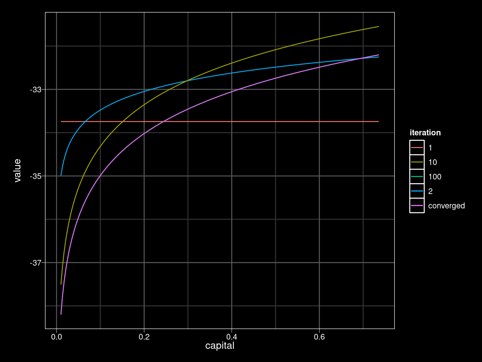

Policy Function

## Warning: `panel.margin` is deprecated. Please use `panel.spacing` property
## instead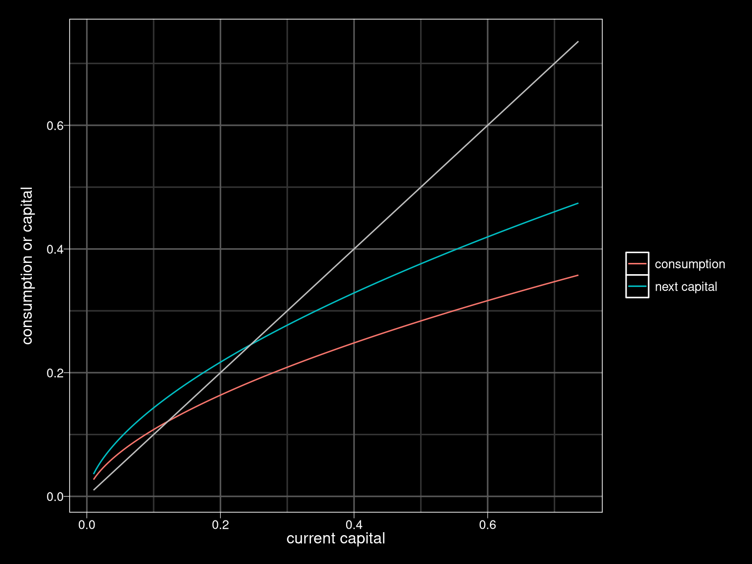

Discrete Controls

• Dynamic programming especially useful for discrete controls
  • No derivatives
  • Binary choice for \(T\) periods \(\leadsto\) \(2^T\) possible combinations of choices
  • Form of policy function often easy to guess (threshold rule)

Example: Investment Option

• Each period: choose invest or not
• Cost \(I\)
• Payoff \(z_t \in [0,B]\) i.i.d with pdf \(f\) and cdf \(F\)
• Bellman equation \[ V(z) = \max\{ z- I , \beta \int V(z') f(z') dz'\} \]

Example: Growth with random productivity

• Production \(A k^\alpha\)
• \(A\) follows a Markov process
• Bellman equation \[ \begin{aligned} V(k_t, A_t) = & \max_{c_t, k_{t+1}} \log (c_t) + \delta \Er[V(k_{t+1}, A_{t+1}) | A_t] \\ & \text{ s.t. } c_t + k_{t+1} = A_t k_t^\alpha \end{aligned} \]