Machine Learning and causal inference

24 September, 2018

This work is licensed under a Creative Commons Attribution-ShareAlike 4.0 International License.

\[ \def\indep{\perp\!\!\!\perp} \def\Er{\mathrm{E}} \def\R{\mathbb{R}} \def\En{{\mathbb{E}_n}} \def\Pr{\mathrm{P}} \newcommand{\norm}[1]{\left\Vert {#1} \right\Vert} \newcommand{\abs}[1]{\left\vert {#1} \right\vert} \DeclareMathOperator*{\argmax}{arg\,max} \DeclareMathOperator*{\argmin}{arg\,min} \]

Introduction

These notes will examine the incorportion of machine learning methods in classic econometric techniques for estimating causal effects. More specifally, we will focus on estimating treatment effects using matching and instrumental variables. In these estimators (and many others) there is a low-dimensional parameter of interest, such as the average treatment effect, but estimating it requires also estimating a potentially high dimensional nuisance parameter, such as the propensity score. Machine learning methods were developed for prediction with high dimensional data. It is then natural to try to use machine learning for estimating high dimensional nuisance parameters. Care must be taken when doing so though because the flexibility and complexity that make machine learning so good at prediction also pose challenges for inference.

About this document

This document was created using Rmarkdown. The code is available in the course github repository. The same document generates both the slides and these notes. The contents of the slides are reproduced here with a white background. Additional information has a beige background. Example code has a grey background. Display of code is toggleable. Divs, like this one, are red.

If you want to print this document, printing works reasonably with Chrome, but not Firefox.

Example: partially linear model

\[ y_i = \theta d_i + f(x_i) + \epsilon_i \]

Interested in \(\theta\)
Assume \(\Er[\epsilon|d,x] = 0\)
Nuisance parameter \(f()\)
E.g. Donohue and Levitt (2001)

The simplest example of the setting we will analyze is a partially linear model. We have some regressor of interest, \(d\), and we want to estimate the effect of \(d\) on \(y\). We have a rich enough set of controls that we are willing to believe that \(E[\epsilon|d,x] = 0\). \(d_i\) and \(y_i\) are scalars, while \(x_i\) is a vector. We are not interested in \(x\) per se, but we need to include it to avoid omitted variable bias.

Typical applied econometric practice would be to choose some transfrom of \(x\), say \(X = T(x)\), where \(X\) could be some subset of \(x\), along with interactions, powers, and so on. Then estimate a linear regression \[ y = \theta d + X'\beta + \epsilon \] and then perhaps also report results for a handful of different choices of \(T(x)\).

Some downsides to the typical applied econometric practice include:

The choice of T is arbitrary, which opens the door to specification searching and p-hacking.
If \(x\) is high dimensional, and \(X\) is low dimensional, a poor choice will lead to omitted variable bias. Even if \(x\) is low dimensional, if \(f(x)\) is poorly approximated by \(X'\beta\), there will be omitted variable bias.

In some sense, machine learning can be thought of as a way to choose \(T\) is an automated and data-driven way. There will be still be a choice of machine learning method and often tuning parameters for that method, so some arbitrary decisions remain. Hopefully though these decisions have less impact.

You may already be familiar with traditional nonparametric econometric methods like series / sieves and kernels. These share much in common with machine learning. What makes machine learning different that traditional nonparametric methods? Machine learning methods appear to have better predictive performance, and arguably more practical data-driven methods to choose tuning parameters. Machine learning methods can deal with high dimensional \(x\), while traditional nonparametric methods focus on situations with low dimensional \(x\).

Example : Effect of abortion on crime

Donohue and Levitt (2001) estimate a regression of state crime rates on crime type relevant abortion rates and controls, \[ y_{it} = \theta a_{it} + x_{it}'\beta + \delta_i + \gamma_t + \epsilon_{it}. \] \(a_{it}\) is a weighted average of lagged abortion rates in state \(i\), with the weight on the \(\ell\)th lag equal to the fraction of age \(\ell\) people who commit a given crime type. The covariates \(x\) are the log of lagged prisoners per capita, the log of lagged police per capita, the unemployment rate, per-capita income, the poverty rate, AFDC generosity at time t − 15, a dummy for concealed weapons law, and beer consumption per cap. Alexandre Belloni, Chernozhukov, and Hansen (2014a) reanalyze this setup using lasso to allow a more flexible specification of controls. They allow for many interactions and quadratic terms, leading to 284 controls.

Example: Matching

Binary treatment \(d_i \in \{0,1\}\)
Potential outcomes \(y_i(0), y_i(1)\), observe \(y_i = y_i(d_i)\)
Interested in average treatment effect : \(\theta = \Er[y_i(1) - y_i(0)]\)
Covariates \(x_i\)
Assume unconfoundedness : \(d_i \indep y_i(1), y_i(0) | x_i\)
E.g. Connors et al. (1996)

Example: Matching

Estimatable formulae for ATE : \[ \begin{align*} \theta = & \Er\left[\frac{y_i d_i}{\Pr(d = 1 | x_i)} - \frac{y_i (1-d_i)}{1-\Pr(d=1|x_i)} \right] \\ \theta = & \Er\left[\Er[y_i | d_i = 1, x_i] - \Er[y_i | d_i = 0 , x_i]\right] \\ \theta = & \Er\left[ \begin{array}{l} d_i \frac{y_i - \Er[y_i | d_i = 1, x_i]}{\Pr(d=1|x_i)} - (1-d_i)\frac{y_i - \Er[y_i | d_i = 0, x_i]}{1-\Pr(d=1|x_i)} + \\ + \Er[y_i | d_i = 1, x_i] - \Er[y_i | d_i = 0 , x_i]\end{array}\right] \end{align*} \]

All the expectations in these three formulae involve observable data. Thus, we can form an estimate of \(\theta\) be replacing the expectations and conditional expectations with appropriate estimators. For example, to use the first formula, we could estimate a logit model for the probability of treatment, \[ \hat{\Pr}(d=1|x_i) = \frac{e^{X_i' \hat{\beta}}}{1+e^{X_i'\hat{\beta}}} \] where, as above, \(X\) is a some chosen transformation of \(x_i\). Then we simply take an average to estimate \(\theta\). \[ \hat{\theta} = \frac{1}{n} \sum_{i=1}^n \frac{y_i d_i}{\hat{\Pr}(d=1|x_i)} - \frac{y_i(1-d_i)} {1-\hat{\Pr}(d=1|x_i)} \] As in the partially linear model, estimating the parameter of interest, \(\theta\), requires estimating a potentially high dimensional nuisance parameter, in this case \(\hat{\Pr}(d=1|x)\). Similarly, the second expression would require estimating conditional expectations of \(y\) as nuisance parameters. The third expression requires estimating both conditional expecations of \(y\) and \(d\).

The third expression might appear needlessly complicated, but we will see later that it has some desirable properties that will make using it essential when very flexible machine learning estimators for the conditional expectations are used.

The origin of the name “matching” can be seen in the second expression. One way to estimate that expression would be to take each person in the treatment group, find someone with the same (or nearly the same) \(x\) in the control group, difference the outcome of this matched pair, and then average over the whole sample. (Actually this gives the average treatment effect on the treated. For the ATE, you would also have to do the same with roles of the groups switched and average all the differences.) When \(x\) is multi-dimensional, there is some ambiguity about what it means for two \(x\) values to be nearly the same. An important insight of Rosenbaum and Rubin (1983) is that it is sufficient to match on the propensity score, \(P(d=1|x)\), instead.

Example: effectiveness of heart catheterization

Connors et al. (1996) use matching to estimate the effectiveness of heart catheterization in critically ill patients. Their dataset contains 5735 patients and 72 covariates. Athey et al. (2017) reanalyze this data using a variety of machine learning methods.

References: Imbens (2004) reviews the traditional econometric literature on matching. Imbens (2015) focuses on practical advice for matching and includes a brief mention of incorporating machine learning.

Both the partially linear model and treatment effects model can be extended to situations with endogeneity and instrumental variables.

Example: IV

\[ \begin{align*} y_i = & \theta d_i + f(x_i) + \epsilon_i \\ d_i = & g(x_i, z_i) + u_i \end{align*} \]

Interested in \(\theta\)
Assume \(\Er[\epsilon|x,z] = 0\), \(\Er[u|x,z]=0\)
Nuisance parameters \(f()\), \(g()\)
E.g. Angrist and Krueger (1991)

Most of the remarks about the partially linear model also apply here.

Hartford et al. (2017) estimate a generalization of this model with \(y_i = f(d_i, x_i) +\epsilon\) using deep neural networks.

Example : compulsory schooling and earnings

Angrist and Krueger (1991) use quarter of birth as an instrument for years of schooling to estimate the effect of schooling on earnings. Since compulsory schooling laws typically specify a minimum age at which a person can leave school instead of a minimum years of schooling, people born at different times of the year can be required to complete one more or one less year of schooling. Compulsory schooling laws and their effect on attained schooling can vary with state and year. Hence, Angrist and Krueger (1991) considered specifying \(g(x,z)\) as all interactions of quarter of birth, state, and year dummies. Having so many instruments leads to statistical problems with 2SLS.

Example: LATE

Binary instrumet \(z_i \in \{0,1\}\)
Potential treatments \(d_i(0), d_i(1) \in \{0,1\}\), \(d_i = d_i(Z_i)\)
Potential outcomes \(y_i(0), y_i(1)\), observe \(y_i = y_i(d_i)\)
Covariates \(x_i\)
\((y_i(1), y_i(0), d_i(1), d_i(0)) \indep z_i | x_i\)
Local average treatment effect: \[ \begin{align*} \theta = & \Er\left[\Er[y_i(1) - y_i(0) | x, d_i(1) > d_i(0)]\right] \\ = & \Er\left[\frac{\Er[y|z=1,x] - \Er[y|z=0,x]} {\Er[d|z=1,x]-\Er[d|z=0,x]} \right] \end{align*} \]

General setup

Parameter of interest \(\theta \in \R^{d_\theta}\)
Nuisance parameter \(\eta \in T\)
Moment conditions \[ \Er[\psi(W;\theta_0,\eta_0) ] = 0 \in \R^{d_\theta} \] with \(\psi\) known
Estimate \(\hat{\eta}\) using some machine learning method
Estimate \(\hat{\theta}\) from \[ \En[\psi(w_i;\hat{\theta},\hat{\eta}) ] = 0 \]

Example: partially linear model

\[ y_i = \theta_0 d_i + f_0(x_i) + \epsilon_i \]

Compare the estimates from
1. \(\En[d_i(y_i - \tilde{\theta} d_i - \hat{f}(x_i)) ] = 0\)
and
1. \(\En[(d_i - \hat{m}(x_i))(y_i - \hat{\mu}(x_i) - \theta (d_i - \hat{m}(x_i)))] = 0\)
where \(m(x) = \Er[d|x]\) and \(\mu(y) = \Er[y|x]\)

Example: partially linear model In the partially linear model,

\[ y_i = \theta_0 d_i + f_0(x_i) + \epsilon_i \]

we can let \(w_i = (y_i, x_i)\) and \(\eta = f\). There are a variety of candidates for \(\psi\). An obvious (but flawed) one is \(\psi(w_i; \theta, \eta) = (y_i - \theta_0 d_i - f_0(x_i))d_i\). With this choice of \(\psi\), we have

\[ \begin{align*} 0 = & \En[d_i(y_i - \hat{\theta} d_i - \hat{f}(x_i)) ] \\ \hat{\theta} = & \En[d_i^2]^{-1} \En[d_i (y_i - \hat{f}(x_i))] \\ (\hat{\theta} - \theta_0) = & \En[d_i^2]^{-1} \En[d_i \epsilon_i] + \En[d_i^2]^{-1} \En[d_i (f_0(x_i) - \hat{f}(x_i))] \end{align*} \]

The first term of this expression is quite promising. \(d_i\) and \(\epsilon_i\) are both finite dimensional random variables, so a law of large numbers will apply to \(\En[d_i^2]\), and a central limit theorem would apply to \(\sqrt{n} \En[d_i \epsilon_i]\). Unfortunately, the second expression is problematic. To accomodate high dimensional \(x\) and allow for flexible \(f()\), machine learning estimators must introduce some sort of regularization to control variance. This regularization also introduces some bias. The bias generally vanishes, but at a slower than \(\sqrt{n}\) rate. Hence

\[ \sqrt{n} \En[d_i (f_0(x_i) - \hat{f}(x_i))] \to \infty. \]

To get around this problem, we must modify our estimate of \(\theta\). Let \(m(x) = \Er[d|x]\) and \(\mu(y) = \Er[y|x]\). Let \(\hat{m}()\) and \(\hat{\mu}()\) be some estimates. Then we can estimate \(\theta\) by partialling out:

\[ \begin{align*} 0 = & \En[(d_i - \hat{m}(x_i))(y_i - \hat{\mu}(x_i) - \theta (d_i - \hat{m}(x_i)))] \\ \hat{\theta} = & \En[(d_i -\hat{m}(x_i))^2]^{-1} \En[(d_i - \hat{m}(x_i))(y_i - \hat{\mu}(x_i))] \\ (\hat{\theta} - \theta_0) = & \En[(d_i -\hat{m}(x_i))^2]^{-1} \left(\En[(d_i - \hat{m}(x_i))\epsilon_i] + \En[(d_i - \hat{m}(x_i))(\mu(x_i) - \hat{\mu}(x_i))] \right) \\ = & \En[(d_i -\hat{m}(x_i))^2]^{-1} \left( a + b +c + d \right) \end{align*} \]

where

\[ \begin{align*} a = & \En[(d_i -m(x_i))\epsilon_i] \\ b = & \En[(m(x_i)-\hat{m}(x_i))\epsilon_i] \\ c = & \En[v_i(\mu(x_i) - \hat{\mu}(x_i))] \\ d = & \En[(m(x_i) - \hat{m}(x_i))(\mu(x_i) - \hat{\mu}(x_i))] \end{align*} \]

with \(v_i = d_i - \Er[d_i | x_i]\). The term \(a\) is well behaved and \(\sqrt{n}a \leadsto N(0,\Sigma)\) under standard conditions. Although terms \(b\) and \(c\) appear similar to the problematic term in the initial estimator, they are better behaved because \(\Er[v|x] = 0\) and \(\Er[\epsilon|x] = 0\). This makes it possible, but difficult to show that \(\sqrt{n}b \to_p = 0\) and \(\sqrt{n} c \to_p = 0\), see e.g. Alexandre Belloni, Chernozhukov, and Hansen (2014a). However, the conditions on \(\hat{m}\) and \(\hat{\mu}\) needed to show this are slightly restrictive, and appropriate conditions might not be known for all estimators. Chernozhukov, Chetverikov, Demirer, Duflo, Hansen, Newey, et al. (2018) describe a sample splitting modification to \(\hat{\theta}\) that allows \(\sqrt{n} b\) and \(\sqrt{n} c\) to vanish under weaker conditions (essentially the same rate condition as needed for \(\sqrt{n} d\) to vanish.)

The last term, \(d\), is a considerable improvement upon the first estimator. Instead of involving the error in one estimate, it now involes the product of the error in two estimates. By the Cauchy-Schwarz inequality, \[ d \leq \sqrt{\En[(m(x_i) - \hat{m}(x_i))^2]} \sqrt{\En[(\mu(x_i) - \hat{\mu}(x_i))^2]}. \] So if the estimates of \(m\) and \(\mu\) converge at rates faster than \(n^{-1/4}\), then \(\sqrt{n} d \to_p 0\). This \(n^{-1/4}\) rate is reached by many machine learning estimators.

Lessons from the example

Need an extra condition on moments – Neyman orthogonality \[ \partial \eta \Er[\psi(W;\theta_0,\eta_0)](\eta-\eta_0) = 0 \]
Want estimators faster than \(n^{-1/4}\) in the prediction norm, \[ \sqrt{\En[(\hat{\eta}(x_i) - \eta(x_i))^2]} \lesssim_P n^{-1/4} \]
Also want estimators that satisfy something like \[ \sqrt{n} \En[(\eta(x_i)-\hat{\eta}(x_i))\epsilon_i] = o_p(1) \]
- Sample splitting will make this easier

References

Matching
- Imbens (2015)
- Imbens (2004)
Surveys on machine learning in econometrics
- Athey and Imbens (2017)
- Mullainathan and Spiess (2017)
- Athey and Imbens (2018)
- Athey et al. (2017)
- Athey and Imbens (2015), Athey and Imbens (2018)
Machine learning
- Breiman and others (2001)
- Friedman, Hastie, and Tibshirani (2009)
- James et al. (2013)
- Efron and Hastie (2016)
Introduction to lasso
- Belloni and Chernozhukov (2011)
- Friedman, Hastie, and Tibshirani (2009) section 3.4
- Chernozhukov, Hansen, and Spindler (2016)
Introduction to random forests
- Friedman, Hastie, and Tibshirani (2009) section 9.2

Neyman orthogonalization
- Chernozhukov, Chetverikov, Demirer, Duflo, Hansen, and Newey (2017)
- Chernozhukov, Hansen, and Spindler (2015)
- Chernozhukov, Chetverikov, Demirer, Duflo, Hansen, Newey, et al. (2018)
- Belloni et al. (2017)
Lasso for causal inference
- Alexandre Belloni, Chernozhukov, and Hansen (2014b)
- Belloni et al. (2012)
- Alexandre Belloni, Chernozhukov, and Hansen (2014a)
- Chernozhukov, Goldman, et al. (2017)
- Chernozhukov, Hansen, and Spindler (2016) hdm R package
Random forests for causal inference
- Athey, Tibshirani, and Wager (2016)
- Wager and Athey (2018)
- Tibshirani et al. (2018) grf R package
- Athey and Imbens (2016)

Introduction to machine learning

Some prediction examples

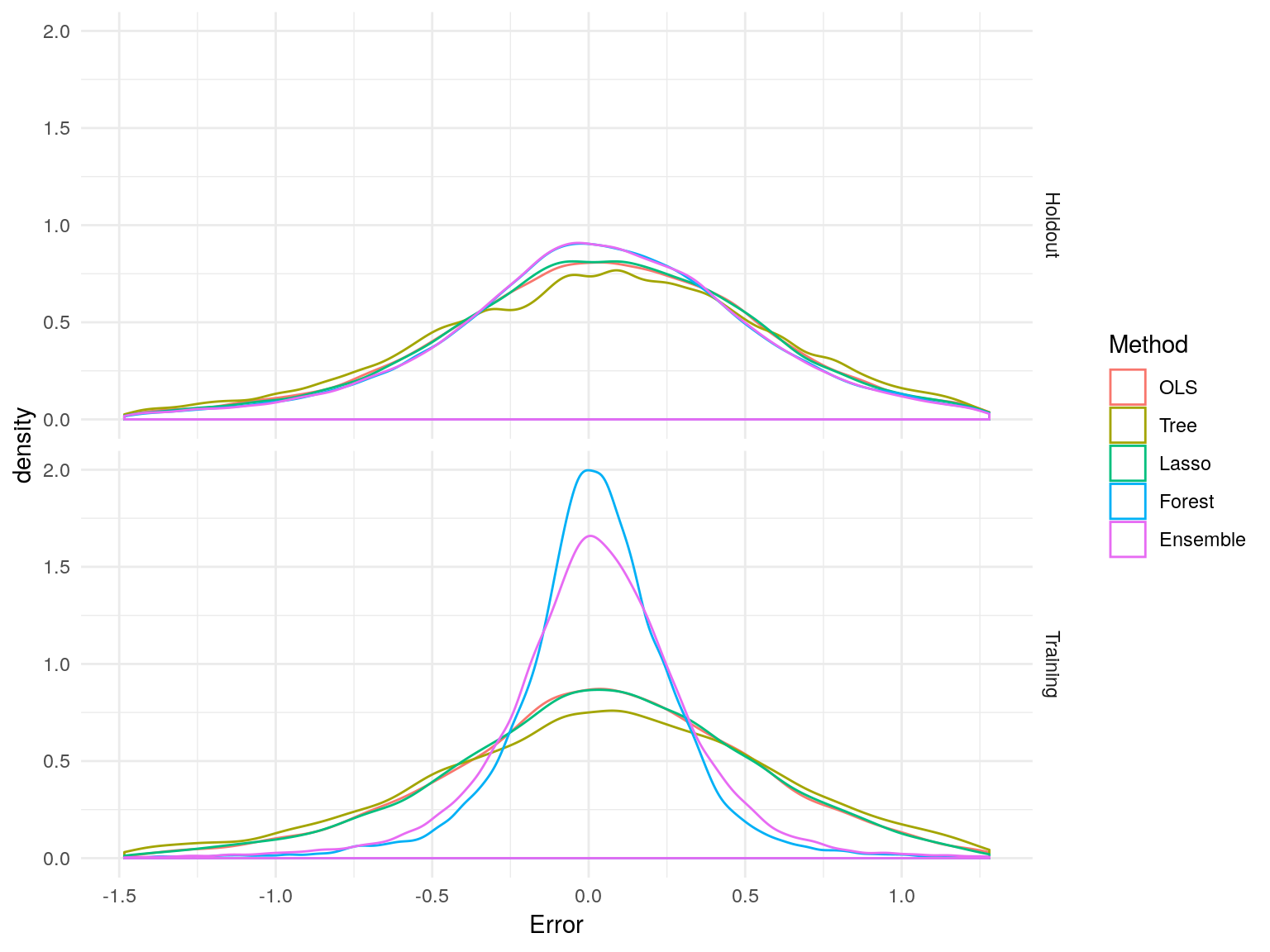
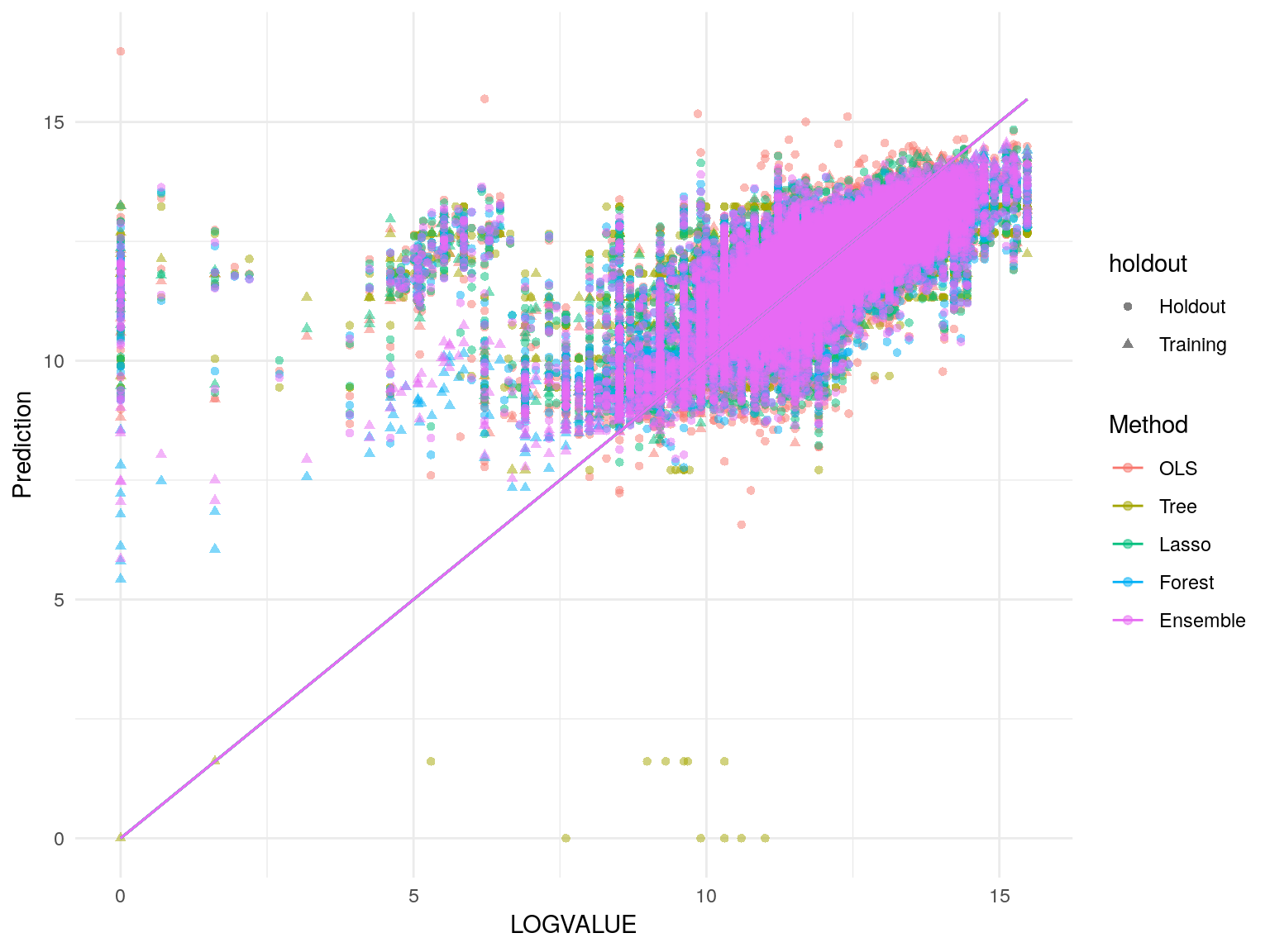
Machine learning is tailored for prediction, let’s look at some data and see how well it works

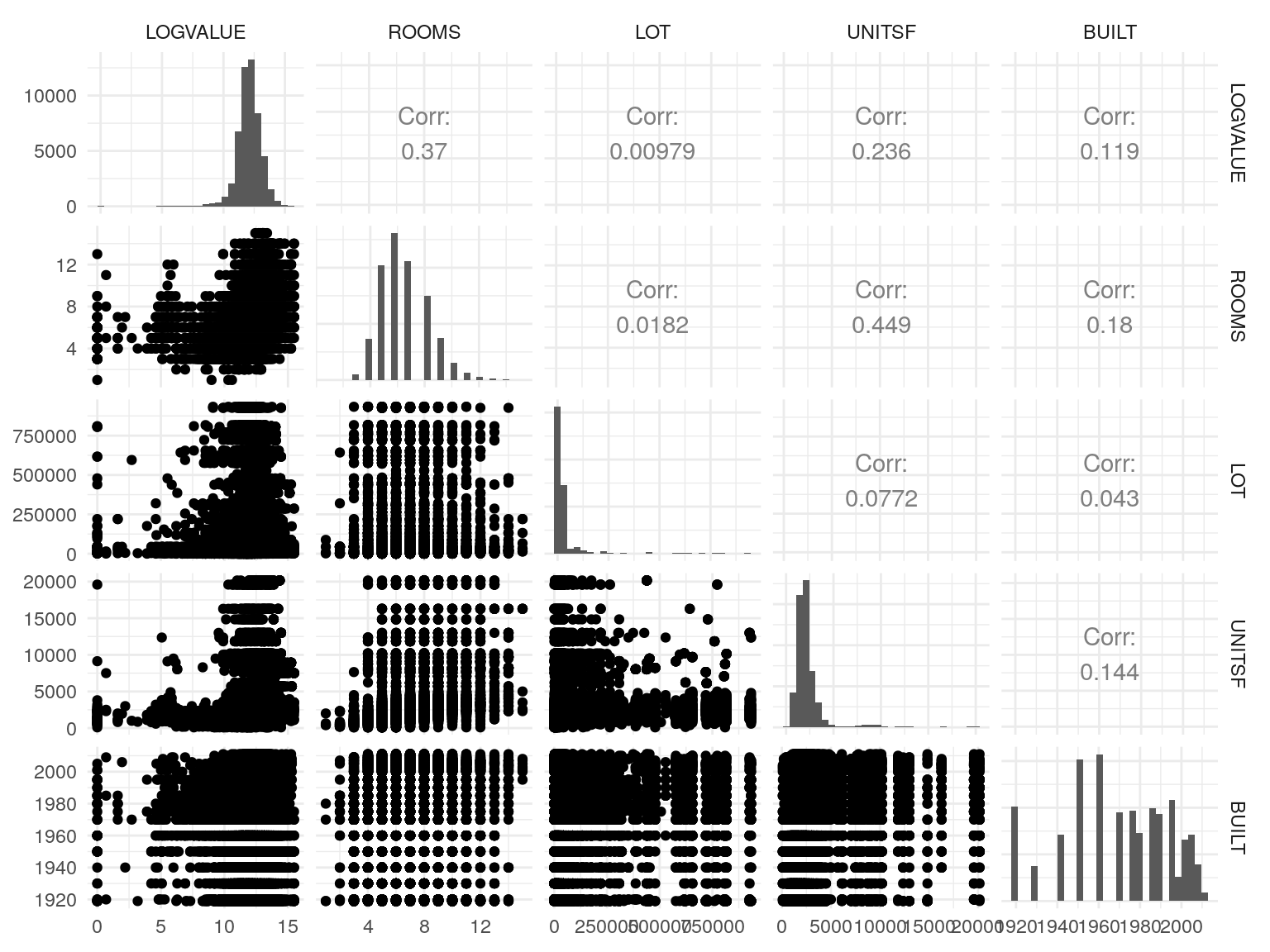
Predicting house prices

Example from Mullainathan and Spiess (2017)
Training on 10000 observations from AHS
Predict log house price using 150 variables
Holdout sample of 41808

AHS variables

##     LOGVALUE     REGION    METRO     METRO3    PHONE      KITCHEN  
##  Min.   : 0.00   1: 5773   1:10499   1:11928   -7: 1851   1:51513  
##  1st Qu.:11.56   2:13503   2: 1124   2:39037   1 :49353   2:  295  
##  Median :12.10   3:15408   3:  202   9:  843   2 :  604            
##  Mean   :12.06   4:17124   4:  103                                 
##  3rd Qu.:12.61             7:39880                                 
##  Max.   :15.48                                                     
##  MOBILTYP   WINTEROVEN WINTERKESP WINTERELSP WINTERWOOD WINTERNONE
##  -1:49868   -8:  133   -8:  133   -8:  133   -8:  133   -8:  133  
##  1 :  927   -7:   50   -7:   50   -7:   50   -7:   50   -7:   50  
##  2 : 1013   1 :  446   1 :  813   1 : 8689   1 :   61   1 :41895  
##             2 :51179   2 :50812   2 :42936   2 :51564   2 : 9730  
##                                                                   
##                                                                   
##  NEWC       DISH      WASH      DRY       NUNIT2    BURNER     COOK     
##  -9:50485   1:42221   1:50456   1:49880   1:44922   -6:51567   1:51567  
##  1 : 1323   2: 9587   2: 1352   2: 1928   2: 2634   1 :   87   2:  241  
##                                           3: 2307   2 :  154            
##                                           4: 1945                       
##                                                                         
##                                                                         
##  OVEN      
##  -6:51654  
##  1 :  127  
##  2 :   27  
##            
##            
##

Performance of different algorithms in predicting housing values
	in sample MSE	in sample R^2	out of sample MSE	out of sample R^2
OLS	0.589	0.473	0.674	0.417
Tree	0.675	0.396	0.758	0.345
Lasso	0.603	0.460	0.656	0.433
Forest	0.166	0.851	0.632	0.454
Ensemble	0.216	0.807	0.625	0.460

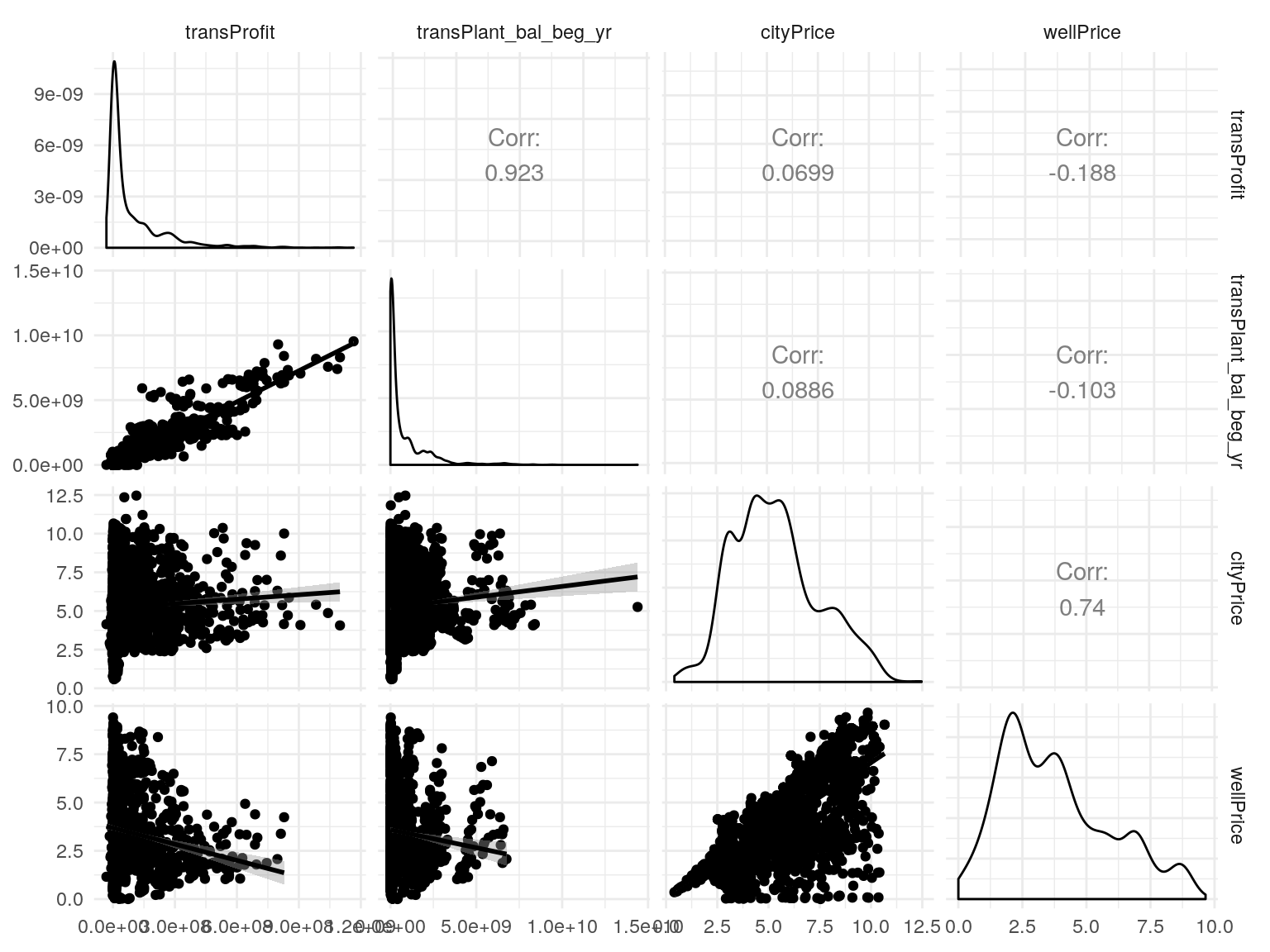
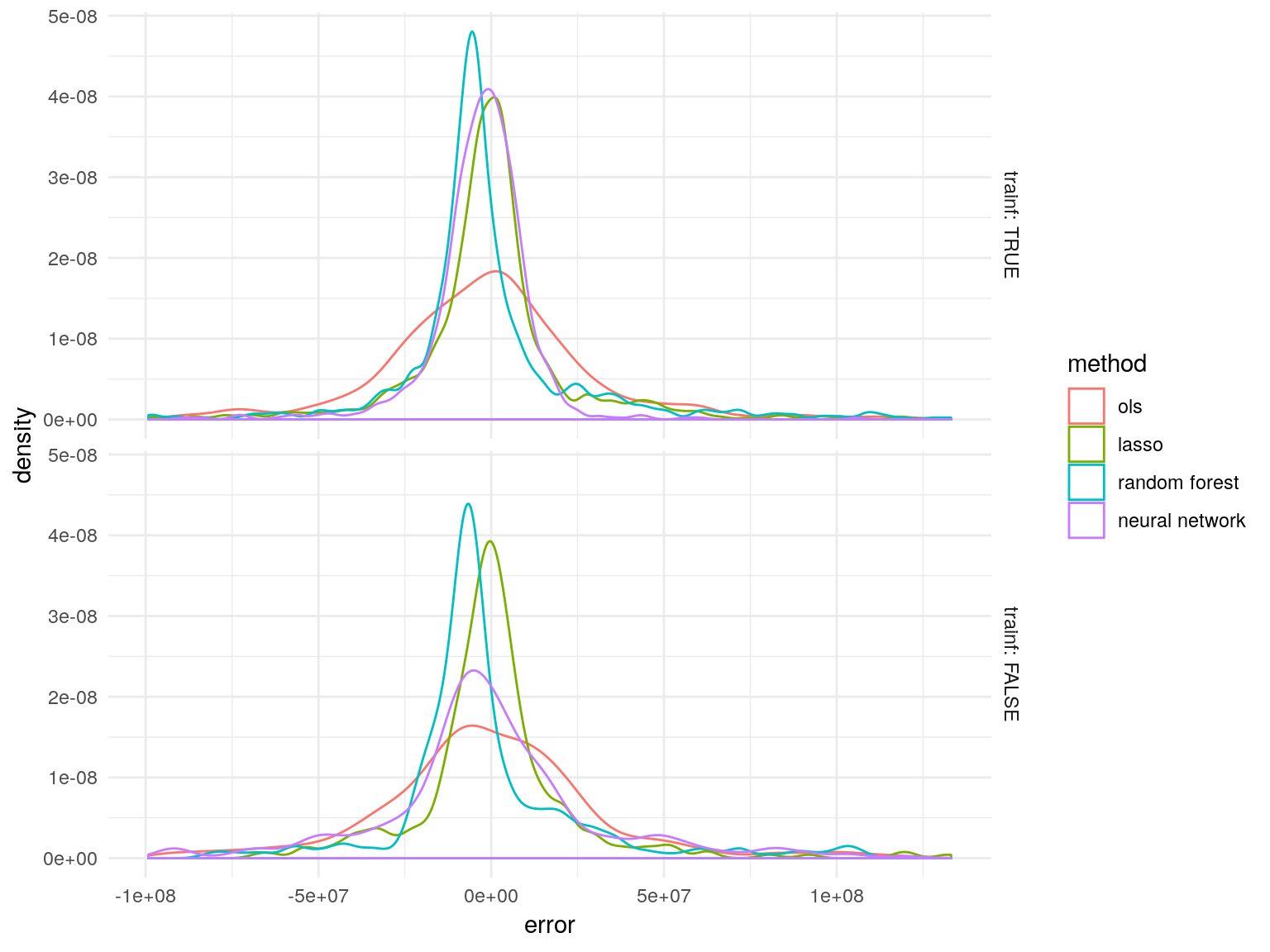
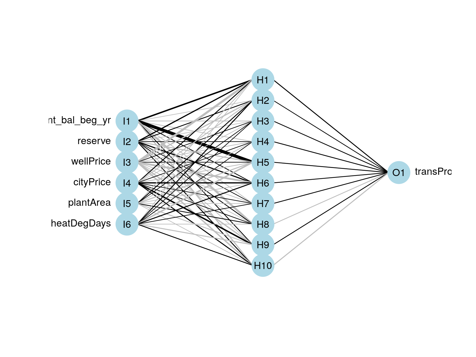
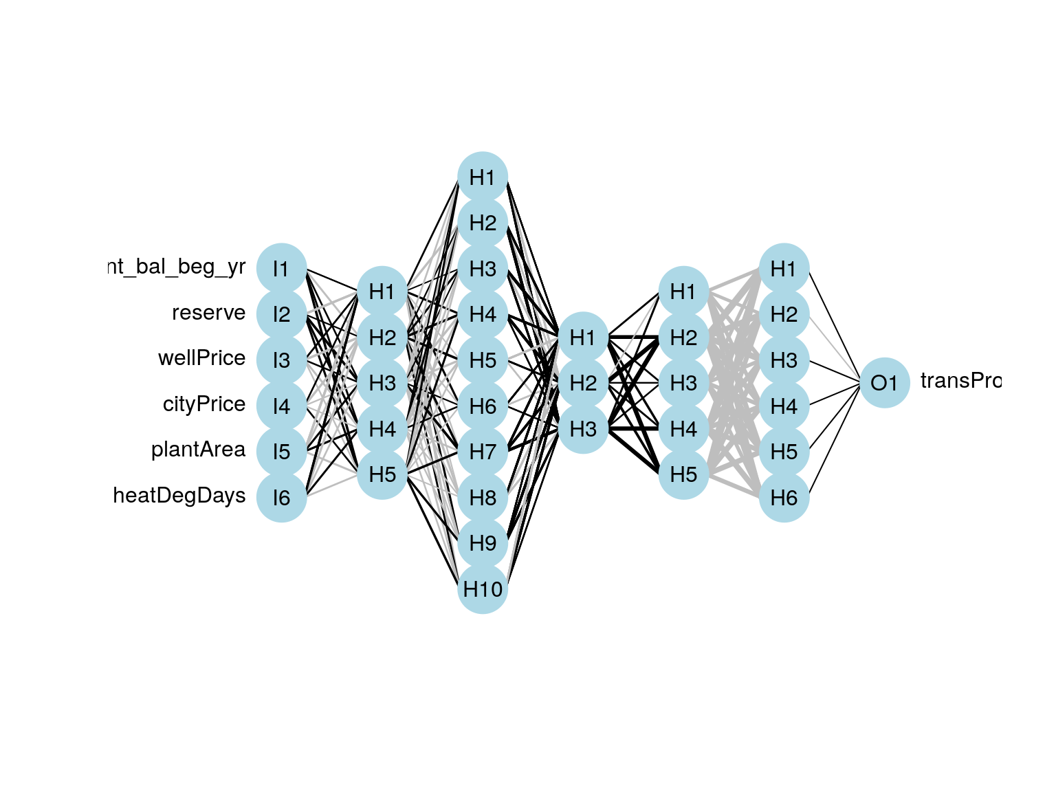
Predicting pipeline revenues

Data on US natural gas pipelines
- Combination of FERC Form 2, EIA Form 176, and other sources, compiled by me
- 1996-2016, 236 pipeline companies, 1219 company-year observations
Predict: \(y =\) profits from transmission of natural gas
Covariates: year, capital, discovered gas reserves, well head gas price, city gate gas price, heating degree days, state(s) that each pipeline operates in

##   transProfit         transPlant_bal_beg_yr   cityPrice      
##  Min.   : -31622547   Min.   :0.000e+00     Min.   : 0.4068  
##  1st Qu.:   2586031   1st Qu.:2.404e+07     1st Qu.: 3.8666  
##  Median :  23733170   Median :1.957e+08     Median : 5.1297  
##  Mean   :  93517513   Mean   :7.772e+08     Mean   : 5.3469  
##  3rd Qu.: 129629013   3rd Qu.:1.016e+09     3rd Qu.: 6.5600  
##  Max.   :1165050214   Max.   :1.439e+10     Max.   :12.4646  
##  NA's   :2817         NA's   :2692          NA's   :1340     
##    wellPrice     
##  Min.   :0.0008  
##  1st Qu.:2.1230  
##  Median :3.4370  
##  Mean   :3.7856  
##  3rd Qu.:5.1795  
##  Max.   :9.6500  
##  NA's   :2637

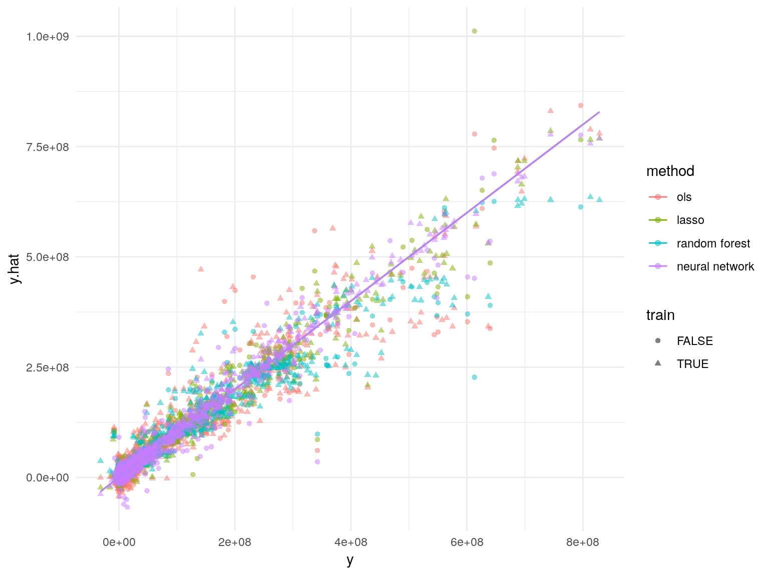
Predicting pipeline revenues : methods

OLS : 67 covariates (year dummies and state(s) create a lot)
Lasso
Random forests
Randomly choose 75% of sample to fit the models, then look at prediction accuracy in remaining 25%

Training sample
	OLS	Lasso	Random forest	Neural Network
relative MSE	0.103	0.030	0.062	0.012
relative MAE	0.260	0.137	0.185	0.094

Hold-out sample
	OLS	Lasso	Random forest	Neural Network
relative MSE	0.142	0.076	0.116	0.079
relative MAE	0.291	0.170	0.236	0.230

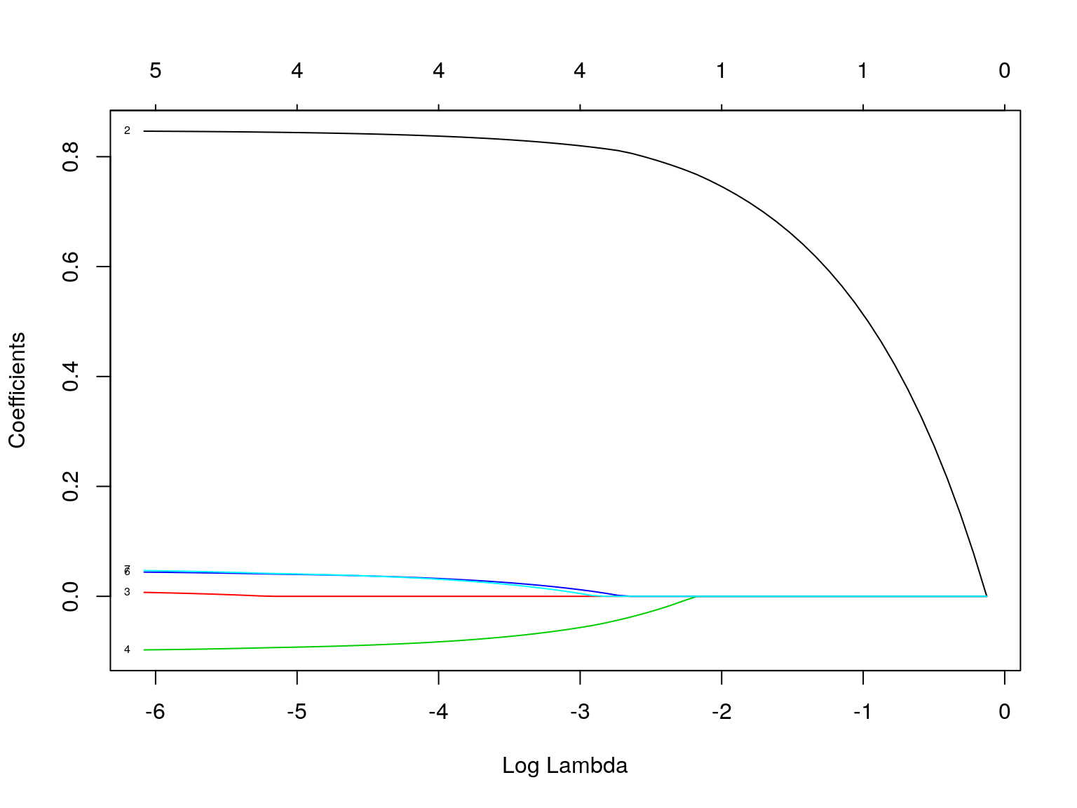
Lasso

Lasso solves a penalized (regularized) regression problem \[ \hat{\beta} = \argmin_\beta \En [ (y_i - x_i'\beta)^2 ] + \frac{\lambda}{n} \norm{ \hat{\Psi} \beta}_1 \]
Penalty parameter \(\lambda\)
Diagonal matrix \(\hat{\Psi} = diag(\hat{\psi})\)
Dimension of \(x_i\) is \(p\) and implicitly depends on \(n\)
- can have \(p >> n\)

We are following the notation used in Chernozhukov, Hansen, and Spindler (2016). Note that this vignette has been updated since it was published in the R Journal. To obtain the most recent version, install the hdm package in R, load it, and then open the vignette.

The choice of penalty (or regularization) parameter, \(\lambda\), is important. When \(\lambda = 0\), Lasso is the same as OLS. As \(\lambda\) increases, the Lasso estimates will shrink toward 0. For large enough \(\lambda\), some components of \(\hat{\beta}\) become exactly 0. As \(\lambda\) increases more, more and more components of \(\hat{\beta}\) will be exactly \(0\).

For some intuition about why Lasso results in some coefficients being zero, note that \[ \hat{\beta}^{lasso} = \argmin_\beta \En [ (y_i - x_i'\beta)^2 ] + \frac{\lambda}{n} \norm{\beta}_1 \] is equivalent to \[\hat{\beta}^{lasso} = \argmin_\beta \En [ (y_i - x_i'\beta)^2 ] \text{ s.t. } \norm{\beta}_1 \leq s \] for some \(s\). In this problem, the boundary of the constraint set will be a diamond. The level sets of the objective will be elipses. Generically, the solution will lie on one of the corners of the \(\norm{\beta}_1 = 1\) set. See Friedman, Hastie, and Tibshirani (2009) or James et al. (2013) for more details.

Most machine learning methods involve some form of regularization with an associated regularization parameter. In choosing the regularization parameter, we face a bias-variance tradeoff. As \(\lambda\) increases, variance decreases, but bias increases.

Machine learning algorithms typically choose regularization parameters through cross-validation. Although cross-validation leads to good predictive performance, the statistical properties are not always known. Chernozhukov, Hansen, and Spindler (2016) say, “In high dimensional settings cross-validation is very popular; but it lacks a theoretical justification for use in the present context.” However, there has been some recent progress on convergence rates for Lasso with cross-validation, see Chetverikov, Liao, and Chernozhukov (2016).

The diagonal matrix \(\hat{\Psi}\) is used to make the estimator invariant to scaling of \(x_i\), and to allow for heteroskedasticity. If reading about Lasso or using code from other authors, be careful some do not include \(\hat{\Psi}\) and use \(\lambda\) instead of \(\frac{\lambda}{n}\).

Statistical properties of Lasso

Model : \[ y_i = x_i'\beta_0 + \epsilon_i \]
- \(\Er[x_i \epsilon_i] = 0\)
- \(\beta_0 \in \R^n\)
- \(p\), \(\beta_0\), \(x_i\), and \(s\) implicitly depend on \(n\)
- \(\log p = o(n^{1/3})\)
  - \(p\) may increase with \(n\) and can have \(p>n\)
Sparsity \(s\)
- Exact : \(\norm{\beta_0}_0 = s = o(n)\)
- Approximate : \(|\beta_{0,j}| < Aj^{-a}\), \(a > 1/2\), \(s \propto n^{1/(2a)}\)

\(\norm{\beta}_0\) is the number of non-zero components of \(\beta\).

The approximate sparsity setting means if \(|\beta_{0,j}| < Aj^{-a}\), then, there exists a sparse approximation, say \(\beta_{a}\), with \(s\) nonzero elements, such that the approximation error, \[ \En[(x_i'(\beta_a - \beta_0))^2] = c_s^2 \] will vanish quickly if \(s \propto n^{1/2a}\). Just how quickly will it vanish? An easy upper bound is \[ \begin{align*} c_s^2 \leq & \En\left[\left( \sum_{j={s+1}}^p x_ij \beta_{0,j} \right)^2 \right] \\ \leq & \En\left[ \left(\sum_{j={s+1}}^p x_ij A j^{-a} \right)^2 \right] \end{align*} \] To simplify the alegebra, let’s assume \(\En[x_i x_i'] = I_p\), then \[ \begin{align*} c_s^2 \leq & \sum_{j={s+1}}^p A^2 j^{-2a} \\ & \leq \sum_{j={s+1}}^\infty A^2 j^{-2a} = A^2 s^{-2a} \zeta(2a) \\ c_s^2 \lesssim s^{-2a} \end{align*} \] where \(\zeta(2a) = \sum_{j=1}^\infty j^{-2a}\) is the Riemann Zeta function (all that matters here is that \(\zeta(2a)\) is finite for \(2a>1\)). Then if \(s \propto n^{(1+\delta)/2a}\), we would get \(c_s \lesssim n^{-(1+\delta)/2}\). Importantly, \(\sqrt{n} c_s = o(1)\), so in the sort of expansions that we would do to show that \(\hat{\theta}\) is \(\sqrt{n}\) asymptotically normal, the bias term would vanish.

Rate of convergence

With \(\lambda = 2c \sqrt{n} \Phi^{-1}(1-\gamma/(2p))\) \[ \sqrt{\En[(x_i'(\hat{\beta}^{lasso} - \beta_0))^2 ] } \lesssim_P \sqrt{ (s/n) \log (p) }, \]

\[ \norm{\hat{\beta}^{lasso} - \beta_0}_2 \lesssim_P \sqrt{ (s/n) \log (p) }, \]

and

\[ \norm{\hat{\beta}^{lasso} - \beta_0}_1 \lesssim_P \sqrt{ (s^2/n) \log (p) } \]

Constant \(c>1\)
- Small \(\gamma \to 0\) with \(n\), and \(\log(1/\gamma) \lesssim \log(p)\)
- Rank like condition on \(x_i\)
near-oracle rate

In the semiparametric estimation problems that we’re focused on, our object of interest is some finite dimensional parameter \(\theta\) that depends on our data some high dimensional parameter, like \(\beta_0\) in the Lasso. To analyze estimates of \(\hat{\theta}(data, \hat{\beta})\), a key step will be to show that we can replace \(\hat{\beta}\) with \(\beta_0\). The rate of convergence of \(\hat{\beta}\) will be important for making this possible. Thus, the main thing that we care about for the Lasso and other machine learning estimators will be their rates of converagence.

The notation \(A_n \lesssim_P B_n\) is read \(A_n\) is bounded in probability by \(B_n\) and means that for any \(\epsilon>0\), there exists \(M\), \(N\) such that \(\Pr(|A_n/B_n| > M) < \epsilon\) for all \(n > N\). This is also often denoted by \(A_n = O(B_n)\).

These rate results are from Belloni et al. (2012). Since this setup allows \(p>n\), \(x\) cannot be assumed to have full rank. Instead, an assumption about the eigenvalues of \(X'X\) restricted to the nonzero components of \(\beta_0\), plays a similar. See Belloni et al. (2012) for details.

This convergence rate is called the near-oracle rate, because it is nearly as good as what we get if an oracle told us which components of \(\beta_0\) are nonzero. In that case OLS using just those \(s\) components gives the fastest possible rate, which is

\[ \sqrt{\En[(x_i'(\hat{\beta}^{OLS} - \beta_0))^2]} \propto \sqrt{s/n}. \]

Rate of convergence

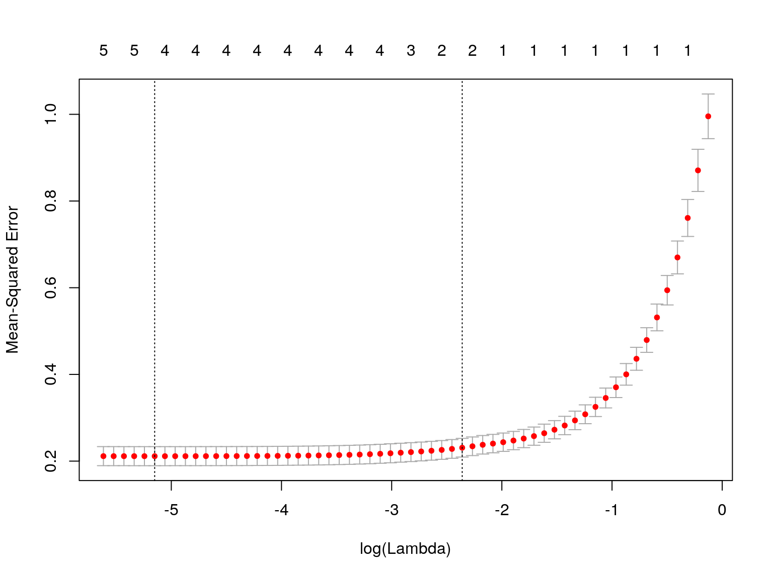
Using cross-validation to choose \(\lambda\) known bounds are worse
- With Gaussian errors: \(\sqrt{\En[(x_i'(\hat{\beta}^{lasso} - \beta_0))^2 ] } \lesssim_P \sqrt{ (s/n) \log (p) } \log(pn)^{7/8}\),
- Without Gaussian error \(\sqrt{\En[(x_i'(\hat{\beta}^{lasso} - \beta_0))^2 ] } \lesssim_P \left( \frac{s \log(pn)^2}{n} \right)^{1/4}\)
- Chetverikov, Liao, and Chernozhukov (2016)

Other statistical properties

Inference on \(\beta\): not the goal in our motivating examples
- Difficult, but some recent results
- See Lee et al. (2016), Taylor and Tibshirani (2017), Caner and Kock (2018)
Model selection: not the goal in our motivating examples
- Under stronger conditions, Lasso correctly selects the nonzero components of \(\beta_0\)
- See Belloni and Chernozhukov (2011)

In the statistics literature on high dimensional and nonparametric estimation, you will come across the terms “adaptive” and “honest.” Adaptivity of an estimator refers to the situation where the rate of convergence depends on some unknown parameter. In the case of Lasso, the sparsity index of the true model, \(s\), is an unknown parameter affecting the rate of convergence. Without knowing or estimating \(s\), Lasso attains the above rate of convergence for a wide range of admissable \(s\). Thus, Lasso is adaptive to the unknown sparsity index.

“Honest” is a property of an inference method. A confidence region is honest if it has correct coverage for a large class of true models. For the Lasso, an honest confidence region would be valid for a wide range of sparsity, \(s\). An honest, adaptive confidence region would be one that is valide for a wide range of \(s\) and whose size shrinks as quickly as if \(s\) were known. Achieving both adaptivity and honesty is impossible in the most general setting. For example, although an \(\ell\) times differentiable function of a \(p\) dimensional variable can be adaptively estimated at rate \(n^{-\ell}{2\ell + p}\), Li (1989) showed that an honest confidence region can contract at most at rate \(n^{-1/4}\) (not adaptive to \(\ell\)). However, an adaptive confidence region can be constructed if further restrictions are placed on the set of possible models, see Nickl and Geer (2013) for such a result for Lasso..

Post-Lasso

Two steps :
1. Estimate \(\hat{\beta}^{lasso}\)
2. \({\hat{\beta}}^{post} =\) OLS regression of \(y\) on components of \(x\) with nonzero \(\hat{\beta}^{lasso}\)
Same rates of convergence as Lasso
Under some conditions post-Lasso has lower bias
- If Lasso selects correct model, post-Lasso converges at the oracle rate

Random forests

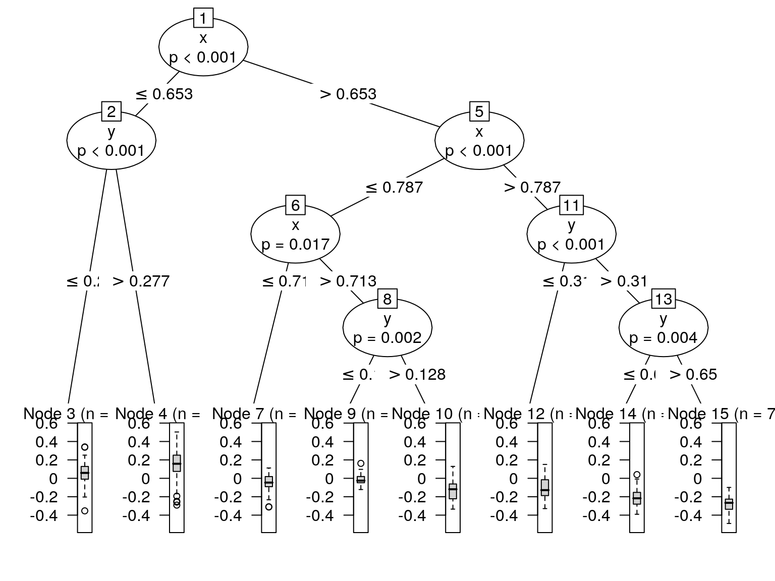
Regression trees

\(y_i \in R\) on \(x_i \in \R^p\)
Want to estimate \(\Er[y | x]\)
Locally constant estimate \[ \hat{t}(x) = \sum_m^M c_m 1\{x \in R_m \} \]
Rectangular regions \(R_m\) determined by tree

Simulated data

Estimated tree

Tree algorithm

For each region, solve \[ \min_{j,s} \left[ \min_{c_1} \sum_{i: x_{i,j} \leq s, x_i \in R} (y_i - c_1)^2 + \min_{c_2} \sum_{i: x_{i,j} > s, x_i \in R} (y_i - c_2)^2 \right] \]
Repeat with \(R = \{x:x_{i,j} \leq s^*\} \cap R\) and \(R = \{x:x_{i,j} \leq s^*\} \cap R\)
Stop when \(|R| =\) some chosen minimum size
Prune tree \[ \min_{tree \subset T} \sum (\hat{f}(x)-y)^2 + \alpha|\text{terminal nodes in tree}| \]

There are many variations on this tree building algorithm. They all share some rule to decide on which variable and where to split. They all have some kind of stopping rule, but not necessarily the same one. For example, some algorithms stop splitting into new branches when the improvement in \(R^2\) becomes small. These trees don’t need subsequent pruning, but also may fail to find later splits that might be important.

As with lasso, regression trees involve some regularization. In the above description, both the minimum leaf size and \(\alpha\) in the pruning step serve as regularization parameters.

A potential advantage of regression trees is that their output might be interpretable, especially if there are not many branches. Some disadvantages are that they often are not very good predictors, and small perturbations in data can lead to seemingly large changes in the tree.

Random forests

Average randomized regression trees
Trees randomized by
- Bootstrap or subsampling
- Randomize branches: \[ \min_{j \in S,s} \left[ \min_{c_1} \sum_{i: x_{i,j} \leq s, x_i \in R} (y_i - c_1)^2 + \min_{c_2} \sum_{i: x_{i,j} > s, x_i \in R} (y_i - c_2)^2 \right] \] where \(S\) is random subset of \(\{1, ..., p\}\)
Variance reduction

Rate of convergence: regression tree

\(x \in [0,1]^p\), \(\Er[y|x]\) Lipschitz in \(x\)
Crude calculation for single tree, let denote \(R_i\) node that contains \(x_i\) \[ \begin{align*} \Er(\hat{t}(x_i) - \Er[y|x_i])^2 = & \overbrace{\Er(\hat{t}(x_i) - \Er[y|x\in R_i])^2}^{variance} + \overbrace{(\Er[y|x \in R_i] - \Er[y|x])^2}^{bias^2} \\ = & O_p(1/m) + O\left(L^2 \left(\frac{m}{n}\right)^{2/p}\right) \end{align*} \] optimal \(m = O(n^{2/(2+p)})\) gives \[ \Er[(\hat{t}(x_i) - \Er[y|x_i])^2] = O_p(n^{\frac{-2}{2+p}}) \]

By a crude calculation, I mean lets treat the tree as fixed. The the variance term is simply from estimating a conditional mean. This analysis could be made more rigorous by assuming the tree was estimated by sample splitting — use half the data to construct the tree and the remaining half to estimate the mean of \(y\) in each node. Athey and Wager, and others, refer to such trees as “honest.” I suppose that this is because sample splitting facilitates honest inference afterward.

The order of the bias term comes from considering the width of the pieces of a \(p\) dimensional cube split evenly into \(n/m\) pieces.

Remember that for our motivating semiparametric problems, we need \(\sqrt{n} \Er[(\hat{t}(x_i) - \Er[y|x_i])^2]\) to vanish. The above rate convergence is too slow for \(p>2\). The calculation of the above was admittedly crude, and may not be exact. However, Stone (1982) showed that if \(\Er[y|x]\) is \(\ell\) times differentiable, the fastest possible rate of convergence for any estimator is \(n^{\frac{-\ell}{2\ell + p}}\). To have any hope of a fast enough rate, we need to assume the function we’re estimating is very smooth (high \(\ell\)), or place some other restriction on the class of functions we allow (like sparsity for the Lasso). Lipschitz continuity is slightly weaker than once differentiable on a compact set, so it should come as no surprise that the rate of convergence would be slow.

Rate of convergence: random forest

Result from Biau (2012)
Assume \(\Er[y|x]=\Er[y|x_{(s)}]\), \(x_{(s)}\) subset of \(s\) variables, then \[ \Er[(\hat{r}(x_i) - \Er[y|x_i])^2] = O_p\left(\frac{1}{m\log(n/m)^{s/2p}}\right) + O_p\left(\left(\frac{m}{n}\right)^{\frac{0.75}{s\log 2}} \right) \] or with optimal \(m\) \[ \Er[(\hat{t}(x_i) - \Er[y|x_i])^2] = O_p(n^{\frac{-0.75}{s\log 2+0.75}}) \]

This result from Biau (2012) assumes the forest is estimated with sample splitting. This avoids the difficult to analyze correlation between the nodes and \(y\).

Wager and Walther (2015) analyze what happens when the same data is used to construct the tree and average in each node. They get a slightly higher upper bound for the variance of \(\frac{\log(p)\log(n)}{m}\). Wager and Walther (2015) also allow \(p\) to increase with \(n\), whereas the previous analysis treated \(p\) as fixed.

These convergence rate results for random forests are not fast enough for our purpose. Does this mean that random forests should not be used in semiparametric estimation? Not necessarily. We’re asking too much of random forests. There is no estimator for an arbitrary Lipschitz function that can have fast enough a rate of convergence. A restriction on the set of possible functions is needed to reduce the approximation bias. With Lasso, the assumption of (approximate) sparsity played that role. Chernozhukov, Chetverikov, Demirer, Duflo, Hansen, Newey, et al. (2018) advise that random forests could be a good choice for semiparametric estimation when the function of interest is “well-approximated by a random forest.” Unfortunately, there does not appear to be a clean mathematical way to describe the class of functions well-approximated by a forest.

Other statistical properties

Pointwise asymptotic normality : Wager and Athey (2018)

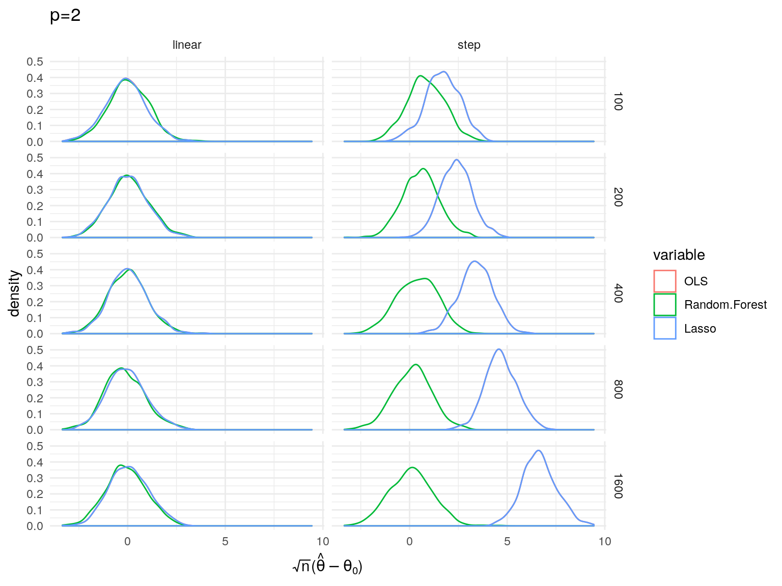
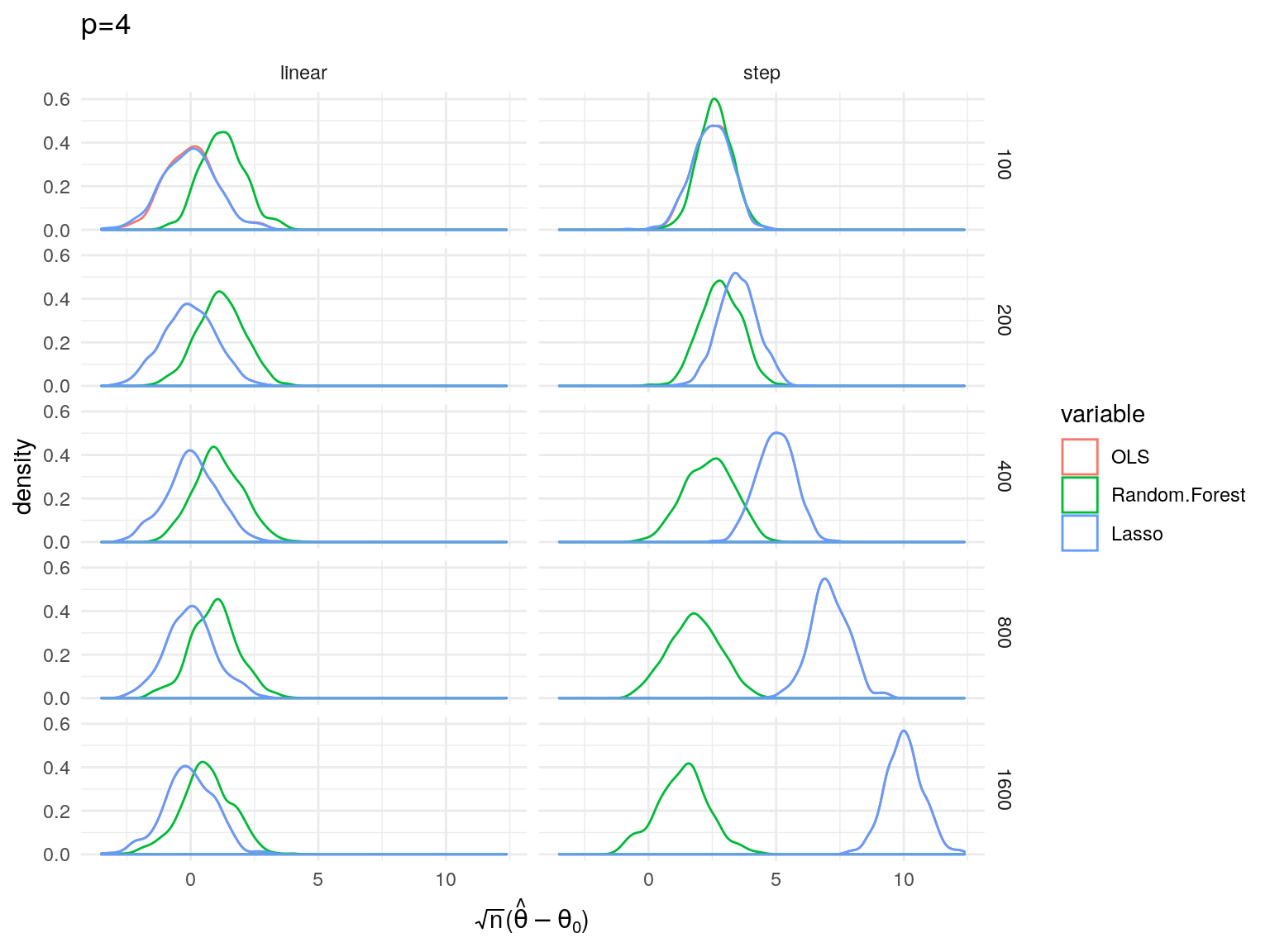
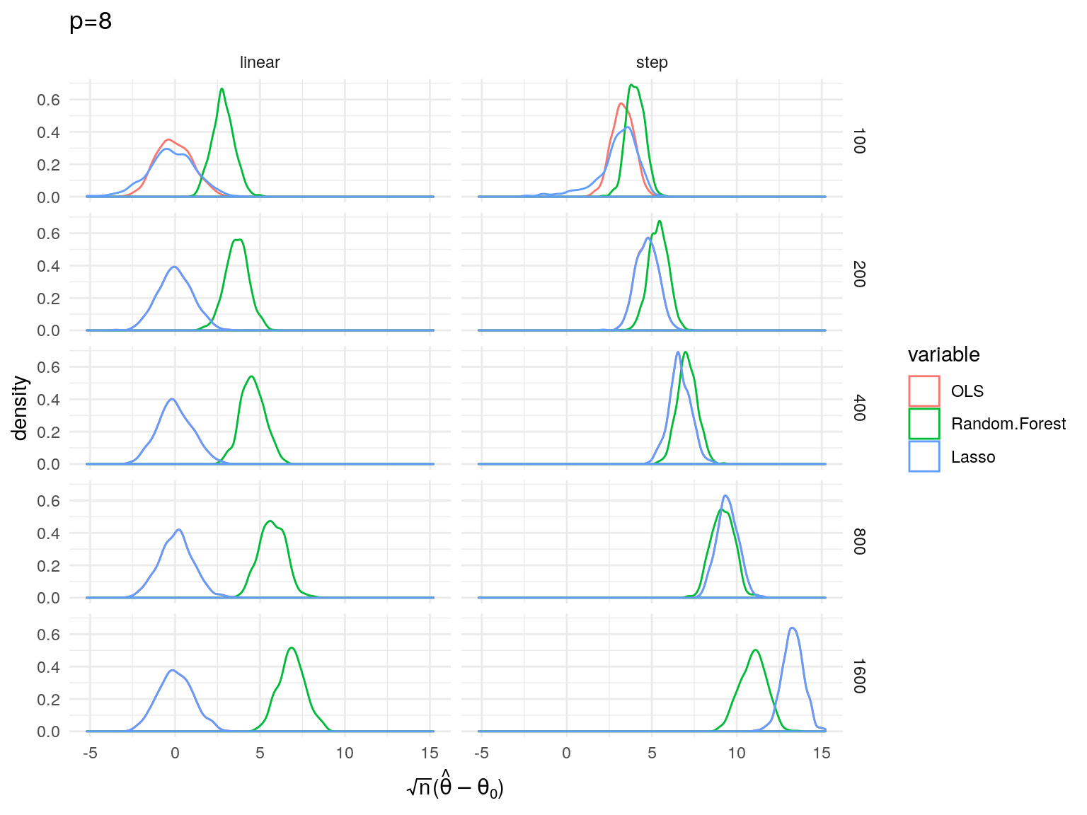
Simulation study

Partially linear model
DGP :
- \(x_i \in \R^p\) with \(x_{ij} \sim U(0,1)\)
- \(d_i = m(x_i) + v_i\)
- \(y_i = d_i\theta + f(x_i) + \epsilon_i\)
- \(m()\), \(f()\) either linear or step functions
Estimate by OLS, Lasso, and random forest
- Lasso & random forest use orthogonal moments \[ \En[(d_i - \hat{m}(x_i))(y_i - \hat{\mu}(x_i) - \theta (d_i - \hat{m}(x_i)))] = 0 \]

The point of this simulation is to see whether the slower convergence rate of random forests matters for the semiparametric problems we have in mind. Our theory results suggest that estimates of \(\theta\) using random forests with \(p>2\) will be asymptotically biased. Specifically, the term \[ d_n = \En[(m(x_i) - \hat{m}(x_i))(\mu(x_i) - \hat{\mu}(x_i))] \] will be \(O_p(n^{\frac{-2}{2+p}})\), so \(\sqrt{n} d_n = O_p(n^{\frac{p-2}{2(2+p)}})\). However, this calculation is only an upper bound on \(d_n\). For a given DGP, \(d_n\) might be smaller.

In this simulation exercise, when \(m()\) and \(f()\) are linear, they are not easy to approximate by a regression tree, so I expect the random forest estimator to behave relatively poorly. OLS and Lasso on the other hand will do very well, and are included mainly as benchmarks. When \(m()\) and \(f()\) are step functions (specifically, \(f(x) = m(x) = \sum_{j=1}^p 1(x_{j}>1/2)\)), I thought they would be well approximated by a regression tree (and random forest). For OLS and Lasso, \(x\) is still only included linearly in the estimation, so those estimators will do poorly in the step function DGP. Throughout the simulation \(p\) is much less than \(n\), so Lasso and OLS will generally give very similar results.

Random forests do not seem to work very well in this context. Even when the functions being estimated are step functions, random forests do not produce a good estimate of \(\theta\). One caveat here is that I was not very careful about the tuning parameters for the random forests. It’s possible that there exists a careful choice of tuning parameters that results in a better estimator.

Research idea: create a generalization of random forests that is adaptive to the smoothness of the function being estimated. Two classic papers on adaptive regression estimators are Speckman (1985) and Donoho and Johnstone (1995). Friedberg et al. (2018) develop a local linear forest estimator. Combining their idea of using forests to form local neighborhoods with a smoothness adaptive variant of kernel or local polynomial regression should lead to a smoothness adaptive forest.

Neural Networks

Target function \(f: \R^p \to \R\)
- e.g. \(f(x) = \Er[y|x]\)
Approximate with single hidden layer neural network : \[ \hat{f}(x) = \sum_{j=1}^r \beta_j (a_j'a_j \vee 1)^{-1} \psi(a_j'x + b_j) \]
- Activation function \(\psi\)
  - Examples: Sigmoid \(\psi(t) = 1/(1+e^{-t})\), Tanh \(\psi(t) = \frac{e^t -e^{-t}}{e^t + e^{-t}}\), Heavyside \(\psi(t) = t 1(t\geq 0)\)
- Weights \(a_j\)
- Bias \(b_j\)
Able to approximate any \(f\), Hornik, Stinchcombe, and White (1989)

Deep Neural Networks

Many hidden layers
- \(x^{(0)} = x\)
- \(x^{(\ell)}_j = \psi(a_j^{(\ell)} x^{(\ell-1)} + b_j^{(\ell)})\)

Rate of convergence

Chen and White (1999)
\(f(x) = \Er[y|x]\) with Fourier representation \[ f(x) = \int e^{i a'x} d\sigma_f(a) \] where \(\int (\sqrt{a'a} \vee 1) d|\sigma_f|(a) < \infty\)
Network sieve : \[ \begin{align*} \mathcal{G}_n = \{ & g: g(x) = \sum_{j=1}^{r_n} \beta_j (a_j'a_j \vee 1)^{-1} \psi(a_j'x + b_j), \\ & \norm{\beta}_1 \leq B_n \} \end{align*} \]

The setup in Chen and White (1999) is more general. They consider estimating both \(f\) and its first \(m\) derivatives. Here, we focus on the case of just estimating \(f\). Chen and White (1999) also consider estimation of functions other than conditional expectations.

The restriction on \(f\) in the second bullet is used to control approximation error. The second bullet says that \(f\) is the inverse Fourier transform of measure \(\sigma_f\). The bite of the restriction on \(f\) comes from the requirement that \(\sigma_f\) be absolutely integral, \(\int (\sqrt{a'a} \vee 1) d|\sigma_f|(a) < \infty\). It would be a good exercise to check whether this restriction is satisfied by some familiar types of functions. Barron (1993) first showed that neural networks approximate this class of functions well, and compares the approximation rate of neural networks to other function approximation results.

Rate of convergence

Estimate \[ \hat{f} = \argmin_{g \in \mathcal{G}_n} \En [(y_i - g(x_i))^2] \]
For fixed \(p\), if \(r_n^{2(1+1/(1+p))} \log(r_n) = O(n)\), \(B_n \geq\) some constant \[ \Er[(\hat{f}(x) - f(x))^2] = O\left((n/\log(n))^{\frac{-(1 + 2/(p+1))} {2(1+1/(p+1))}}\right) \]

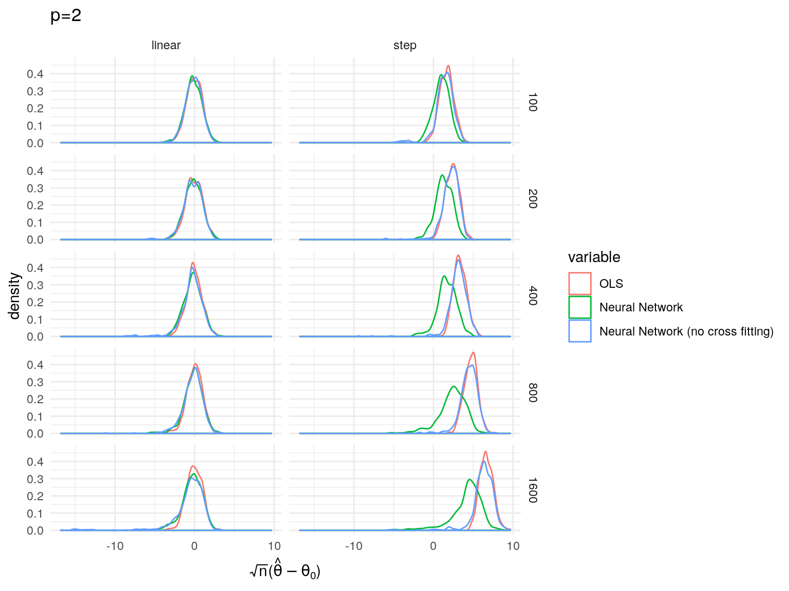
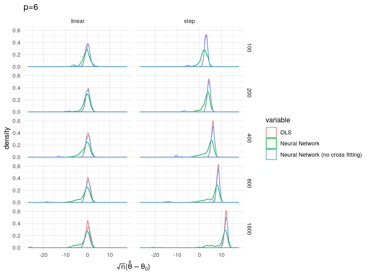
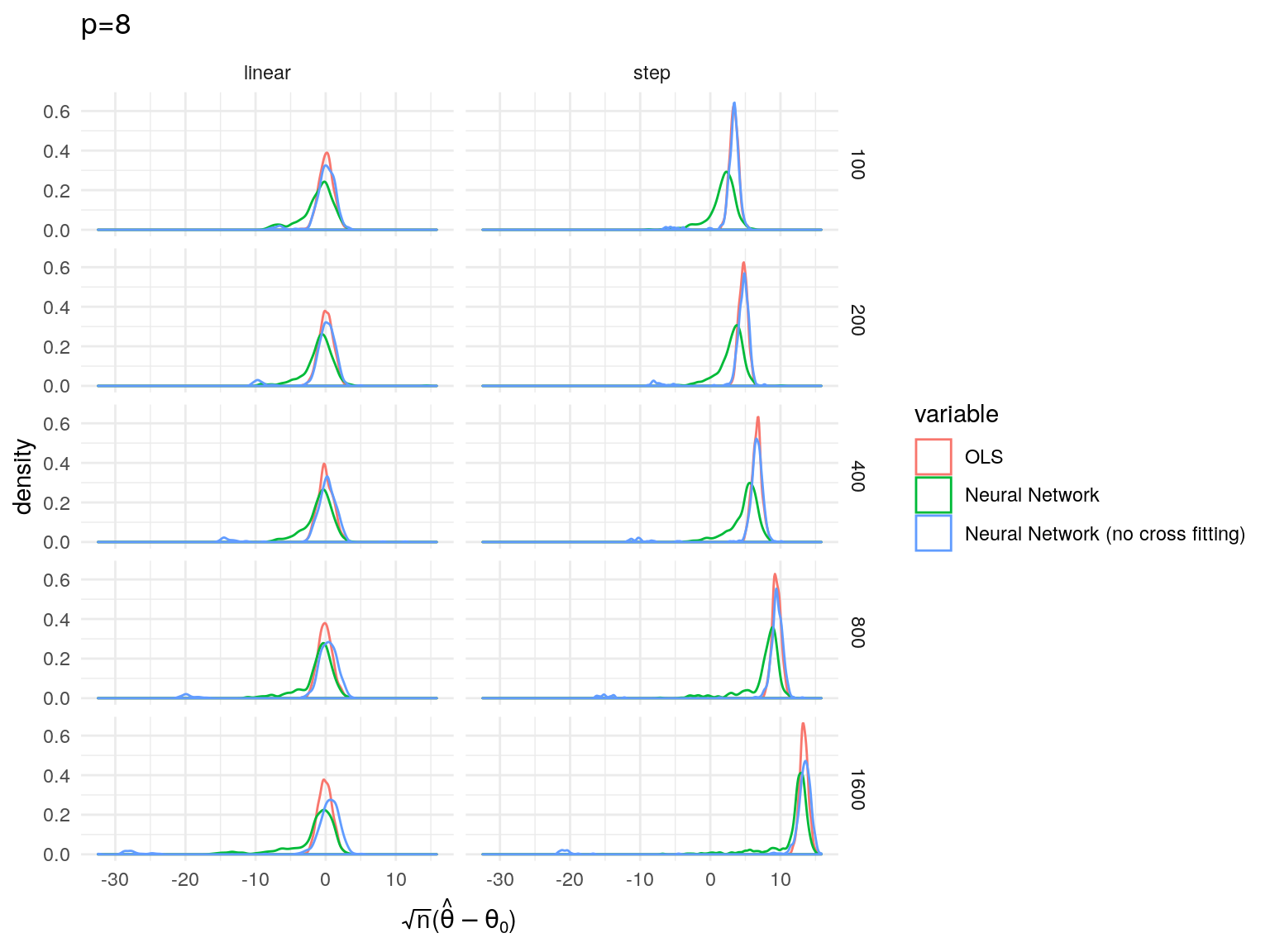
Simulation Study

Same setup as for random forests earlier
Partially linear model
DGP :
- \(x_i \in \R^p\) with \(x_{ij} \sim U(0,1)\)
- \(d_i = m(x_i) + v_i\)
- \(y_i = d_i\theta + f(x_i) + \epsilon_i\)
- \(m()\), \(f()\) either linear or step functions
Estimate by OLS, Neural network with & without cross-fitting
- Using orthogonal moments \[ \En[(d_i - \hat{m}(x_i))(y_i - \hat{\mu}(x_i) - \theta (d_i - \hat{m}(x_i)))] = 0 \]

The performance of the neural network estimator appears okay, but not outstanding in these simulations. In the linear model, the neural network estimator performs slightly worse than OLS. In the step function model, the neural network estimator performs slight better than the misspecified OLS, but neither appears to work well. In both cases, it appears that the neural network estimator produces occassional outliers. I believe that this is related to the fact that the minimization problem defining the neural network is actually very difficult to solve. In the simulation above, I suspect the outlying estimates are due to minimization problems. In the simulations, I simply set \(r_n = n^{1/(2(1+1/(1+p)))}\). It’s likely that a more careful choice of \(r_n\), perhaps using cross-validation, would give better results.

Using machine learning to estimate causal effects

Double debiased machine learning

Chernozhukov, Chetverikov, Demirer, Duflo, Hansen, Newey, et al. (2018), Chernozhukov, Chetverikov, Demirer, Duflo, Hansen, and Newey (2017)
Parameter of interest \(\theta \in \R^{d_\theta}\)
Nuisance parameter \(\eta \in T\)
Moment conditions \[ \Er[\psi(W;\theta_0,\eta_0) ] = 0 \in \R^{d_\theta} \] with \(\psi\) known
Estimate \(\hat{\eta}\) using some machine learning method
Estimate \(\hat{\theta}\) using cross-fitting

Cross-fitting

Randomly partition into \(K\) subsets \((I_k)_{k=1}^K\)
\(I^c_k = \{1, ..., n\} \setminus I_k\)
\(\hat{\eta}_k =\) estimate of \(\eta\) using \(I^c_k\)
Estimator: \[ \begin{align*} 0 = & \frac{1}{K} \sum_{k=1}^K \frac{K}{n} \sum_{i \in I_k} \psi(w_i;\hat{\theta},\hat{\eta}_k) \\ 0 = & \frac{1}{K} \sum_{k=1}^K \En_k[ \psi(w_i;\hat{\theta},\hat{\eta}_k)] \end{align*} \]

Assumptions

Linear score \[ \psi(w;\theta,\eta) = \psi^a(w;\eta) \theta + \psi^b(w;\eta) \]
Near Neyman orthogonality: \[ \lambda_n := \sup_{\eta \in \mathcal{T}_n} \norm{\partial \eta \Er\left[\psi(W;\theta_0,\eta_0)[\eta-\eta_0] \right] } \leq \delta_n n^{-1/2} \]

Assumptions

Rate conditions: for \(\delta_n \to 0\) and \(\Delta_n \to 0\), we have \(\Pr(\hat{\eta}_k \in \mathcal{T}_n) \geq 1-\Delta_n\) and \[ \begin{align*} r_n := & \sup_{\eta \in \mathcal{T}_n} \norm{ \Er[\psi^a(W;\eta)] - \Er[\psi^a(W;\eta_0)]} \leq \delta_n \\ r_n' := & \sup_{\eta \in \mathcal{T}_n} \Er\left[ \norm{ \psi(W;\theta_0,\eta) - \psi(W;\theta_0,\eta_0)}^2 \right]^{1/2} \leq \delta_n \\ \lambda_n' := & \sup_{r \in (0,1), \eta \in \mathcal{T}_n} \norm{ \partial_r^2 \Er\left[\psi(W;\theta_0, \eta_0 + r(\eta - \eta_0)) \right]} \leq \delta_n/\sqrt{n} \end{align*} \]
Moments exist and other regularity conditions

Proof outline:

Let \(\hat{J} = \frac{1}{K} \sum_{k=1}^K \En_k [\psi^a(w_i;\hat{\eta}_k)]\), \(J_0 = \Er[\psi^a(w_i;\eta_0)]\), \(R_{n,1} = \hat{J}-J_0\)
Show: \[ \small \begin{align*} \sqrt{n}(\hat{\theta} - \theta_0) = & -\sqrt{n} J_0^{-1} \En[\psi(w_i;\theta_0,\eta_0)] + \\ & + (J_0^{-1} - \hat{J}^{-1}) \left(\sqrt{n} \En[\psi(w_i;\theta_0,\eta_0)] + \sqrt{n}R_{n,2}\right) + \\ & + \sqrt{n}J_0^{-1}\underbrace{\left(\frac{1}{K} \sum_{k=1}^K \En_k[ \psi(w_i;\theta_0,\hat{\eta}_k)] - \En[\psi(w_i;\theta_0,\eta_0)]\right)}_{R_{n,2}} \end{align*} \]
Show \(\norm{R_{n,1}} = O_p(n^{-1/2} + r_n)\)
Show \(\norm{R_{n,2}}= O_p(n^{-1/2} r_n' + \lambda_n + \lambda_n')\)

Proof outline: Lemma 6.1

Lemma 6.1

If \(\Pr(\norm{X_m} > \epsilon_m | Y_m) \to_p 0\), then \(\Pr(\norm{X_m}>\epsilon_m) \to 0\).
If \(\Er[\norm{X_m}^q/\epsilon_m^q | Y_m] \to_p 0\) for \(q\geq 1\), then \(\Pr(\norm{X_m}>\epsilon_m) \to 0\).
If \(\norm{X_m} = O_p(A_m)\) conditional on \(Y_m\) (i.e. for any \(\ell_m \to \infty\), \(\Pr(\norm{X_m} > \ell_m A_m | Y_m) \to_p 0\)), then \(\norm{X_m} = O_p(A_m)\) unconditionally

Proof outline: \(R_{n,1}\)

\[ R_{n,1} = \hat{J}-J_0 = \frac{1}{K} \sum_k \left( \En_k[\psi^a(w_i;\hat{\eta}_k)] - \Er[\psi^a(W;\eta_0)] \right) \]

\(\norm{\En_k[\psi^a(w_i;\hat{\eta}_k)] - \Er[\psi^a(W;\eta_0)]} \leq U_{1,k} + U_{2,k}\) where \[ \begin{align*} U_{1,k} = & \norm{\En_k[\psi^a(w_i;\hat{\eta}_k)] - \Er[\psi^a(W;\hat{\eta}_k)| I^c_k]} \\ U_{2,k} = & \norm{ \Er[\psi^a(W;\hat{\eta}_k)| I^c_k] - \Er[\psi^a(W;\eta_0)]} \end{align*} \]

Proof outline: \(R_{n,2}\)

\(R_{n,2} = \frac{1}{K} \sum_{k=1}^K \En_k\left[ \psi(w_i;\theta_0,\hat{\eta}_k) - \psi(w_i;\theta_0,\eta_0) \right]\)
\(\sqrt{n} \norm{\En_k\left[ \psi(w_i;\theta_0,\hat{\eta}_k) - \psi(w_i;\theta_0,\eta_0) \right]} \leq U_{3,k} + U_{4,k}\) where

\[ \small \begin{align*} U_{3,k} = & \norm{ \frac{1}{\sqrt{n}} \sum_{i \in I_k} \left( \psi(w_i;\theta_0, \hat{\eta}_k) - \psi(w_i;\theta_0,\eta_0) - \Er[ \psi(w_i;\theta_0, \hat{\eta}_k) - \psi(w_i;\theta_0,\eta_0)] \right) } \\ U_{4,k} = & \sqrt{n} \norm{ \Er[ \psi(w_i;\theta_0, \hat{\eta}_k) | I_k^c] - \Er[\psi(w_i;\theta_0,\eta_0)]} \end{align*} \]

\(U_{4,k} = \sqrt{n} \norm{f_k(1)}\) where

\[ f_k(r) = \Er[\psi(W;\theta_0,\eta_0 + r(\hat{\eta}_k - \eta_0)) | I^c_k] - \Er[\psi(W;\theta_0,\eta_0)] \]

Asymptotic normality

\[ \sqrt{n} \sigma^{-1} (\hat{\theta} - \theta_0) = \frac{1}{\sqrt{n}} \sum_{i=1}^n \bar{\psi}(w_i) + O_p(\rho_n) \leadsto N(0,I) \]

\(\rho_n := n^{-1/2} + r_n + r_n' + n^{1/2} (\lambda_n +\lambda_n') \lesssim \delta_n\)
Influence function \[\bar{\psi}(w) = -\sigma^{-1} J_0^{-1} \psi(w;\theta_0,\eta_0)\]
\(\sigma^2 := J_0^{-1} \Er[\psi(w;\theta_0,\eta_0) \psi(w;\theta_0,\eta_0)'](J_0^{-1})'\)

Creating orthogonal moments

Need \[ \partial \eta\Er\left[\psi(W;\theta_0,\eta_0)[\eta-\eta_0] \right] \approx 0 \]
Given an some model, how do we find a suitable \(\psi\)?

Orthogonal scores via concentrating-out

Original model: \[ (\theta_0, \beta_0) = \argmax_{\theta, \beta} \Er[\ell(W;\theta,\beta)] \]
Define \[ \eta(\theta) = \beta(\theta) = \argmax_\beta \Er[\ell(W;\theta,\beta)] \]
First order condition from \(\max_\theta \Er[\ell(W;\theta,\beta(\theta))]\) is \[ 0 = \Er\left[ \underbrace{\frac{\partial \ell}{\partial \theta} + \frac{\partial \ell}{\partial \beta} \frac{d \beta}{d \theta}}_{\psi(W;\theta,\beta(\theta))} \right] \]

Orthogonal scores via projection

Original model: \(m: \mathcal{W} \times \R^{d_\theta} \times \R^{d_h} \to \R^{d_m}\) \[ \Er[m(W;\theta_0,h_0(Z))|R] = 0 \]
Let \(A(R)\) be \(d_\theta \times d_m\) moment selection matrix, \(\Omega(R)\) \(d_m \times d_m\) weighting matrix, and \[ \begin{align*} \Gamma(R) = & \partial_{v'} \Er[m(W;\theta_0,v)|R]|_{v=h_0(Z)} \\ G(Z) = & \Er[A(R)'\Omega(R)^{-1} \Gamma(R)|Z] \Er[\Gamma(R)'\Omega(R)^{-1} \Gamma(R) |Z]^{-1} \\ \mu_0(R) = & A(R)'\Omega(R)^{-1} - G(Z) \Gamma(R)'\Omega(R)^{-1} \end{align*} \]
\(\eta = (\mu, h)\) and \[ \psi(W;\theta, \eta) = \mu(R) m(W;\theta, h(Z)) \]

Example: average derivative

\(x,y \in \R^1\), \(\Er[y|x] = f_0(x)\), \(p(x) =\) density of \(x\)
\(\theta_0 = \Er[f_0'(x)]\)
Joint objective \[ \min_{\theta,f} \Er\left[ (y - f(x))^2 + (\theta - f'(x)^2) \right] \]
\(f_\theta(x) = \Er[y|x] + \theta \partial_x \log p(x) - f''(x) - f'(x) \partial_x \log p(x)\)
Concentrated objective: \[ \min_\theta \Er\left[ (y - f_\theta(x))^2 + (\theta - f_\theta'(x)^2) \right] \]
First order condition at \(f_\theta = f_0\) gives \[ 0 = \Er\left[ (y - f_0(x))\partial_x \log p(x) + (\theta - f_0'(x)) \right] \]

Example : average derivative with endogeneity

\(x,y \in \R^1\), \(p(x) =\) density of \(x\)
Model : \(\Er[y - f(x) | z] = 0\) \(\theta_0 = \Er[f_0'(x)]\)
Joint objective: \[ \min_{\theta,f} \Er\left[ \Er[y - f(x)|z]^2 + (\theta - f'(x))^2 \right] \]
\(f_\theta(x) = (T^* T)^{-1}\left((T^*\Er[y|z])(x) - \theta \partial_x \log p(x)\right)\)
- where \(T:\mathcal{L}^2_{p} \to \mathcal{L}^2_{\mu_z}\) with \((T f)(z) = \Er[f(x) |z]\)
- and \(T^*:\mathcal{L}^2_{\mu_z} \to \mathcal{L}^2_{p}\) with \((T^* g)(z) = \Er[g(z) |x]\)
Orthogonal moment condition : \[ 0 = \Er\left[ \Er[y - f(x) | z] (T (T^* T)^{-1} \partial_x \log p)(z) + (\theta - f'(x)) \right] \]

The first order condition for \(f\) in the joint objective function is \[ \begin{align*} 0 = \Er \left[ \Er[y-f(x) |z]\Er[v(x)|z] + (\theta - f'(x))(-v'(x)) \right] \end{align*} \] Writing these expectations as integrals, integrating by parts to get rid of \(v'(x)\), and switching the order of integration, gives \[ \begin{align*} 0 = \int_\mathcal{X} v(x)\left( \int_\mathcal{Z} \Er[y - f(x)|z] p(z|x) dz - (\theta-f'(x))\partial_x \log p(x) - f''(x) \right) p(x) dx \end{align*} \] Notice that integrating by parts \(\int f''(x) p(x) dx = \int f' p'(x) dx\) eliminates the terms with \(f'\) and \(f''\), leaving \[ \begin{align*} 0 = \int_\mathcal{X} v(x)\left( \int_\mathcal{Z} \Er[y - f(x)|z] p(z|x) dz - \theta \partial_x \log p(x) \right) p(x) dx \end{align*} \] For this to be \(0\) for all \(v\), we need \[ 0 = \int_\mathcal{Z} \Er[y - f(x)|z] p(z|x) dz - \theta \partial_x \log p(x) \] or equivalently using \(T\) and \(T^*\), \[ 0 = \left(T^*(E[y|z] - T f)\right)(x) - \theta \partial_x \log p(x) \] Note that \(T\) and \(T^*\) are linear, and \(T^*\) is the adjoint of \(T\). Also, identification of \(f\) requires \(T\) is one to one. Hence, if \(f\) is identified, \(T^* T\) is invertible. Therefore, we can solve for \(f\) as: \[ f_\theta(x) = (T^* T)^{-1} \left( (T^* \Er[y |z])(x) - \theta \partial \log p(x) \right) \] Plugging \(f_\theta(x)\) back into the objective function and then differentiating with respect to \(\theta\) gives the orthogonal moment condition on the slide. Verifying that this moment condition is indeed orthogonal is slightly tedious. Writing out some of the expectations as integrals, changing order of integrations, and judiciously factoring out terms, will eventually lead to the desired conclusion.

Carrasco, Florens, and Renault (2007) is an excellent review about estimating \((T^* T)^{-1}\) and the inverses of other linear transformations.

Example: average elasticity

Demand \(D(p)\), quantities \(q\), instruments \(z\) \[\Er[q-D(p) |z] = 0\]
Average elasticity \(\theta \Er[D'(p)/D(p) | z ]\)
Joint objective : \[ \min_{\theta,D} \Er\left[ \Er[q - D(p)|z]^2 + (\theta - D'(p)/D(p))^2 \right] \]

Example: control function

\[ \begin{align*} 0 = & \Er[d - p(x,z) | x,z] \\ 0 = & \Er[y - x\beta - g(p(x,z)) | x,z] \end{align*} \]

Treatment heterogeneity

Potential outcomes model
- Treatment \(d \in \{0,1\}\)
- Potential outcomes \(y(1), y(0)\)
- Covariates \(x\)
- Unconfoundedness or instruments
Objects of interest:
- Conditional average treatment effect \(s_0(x) = \Er[y(1) - y(0) | x]\)
- Range and other measures of spread of conditional average treatment effect
- Most and least affected groups

Fixed, finite groups

\(G_1, ..., G_K\) finite partition of support \((x)\)
Estimate \(\Er[y(1) - y(0) | x \in G_k]\) as above
pros: easy inference, reveals some heterogeneity
cons: poorly chosen partition hides some heterogeneity, searching partitions violates inference

Generic Machine Learning Inference on Heterogenous Treatment Effects in Randomized Experiments

Chernozhukov, Demirer, et al. (2018)
Use machine learning to find partition with sample splitting to allow easy inference
Randomly partition sample into auxillary and main samples
Use any method on auxillary sample to estimate \[S(x) = \widehat{\Er[y(1) - y(0) | x]}\] and \[B(x) = \widehat{\Er[y(0)|x]}\]

Generic Machine Learning Inference on Heterogenous Treatment Effects in Randomized Experiments

Define \(G_k = 1\{\ell_{k-1} \leq S(x) \leq \ell_k\}\)
Use main sample to regress with weights \((P(x)(1-P(X)))^{-1}\) \[ y = \alpha_0 + \alpha_1 B(x) + \sum_k \gamma_k (d-P(X)) 1(G_k) + \epsilon \]
\(\hat{\gamma}_k \to_p \Er[y(1) - y(0) | G_k]\)

Best linear projection of CATE

Randomly partition sample into auxillary and main samples
Use any method on auxillary sample to estimate \[S(x) = \widehat{\Er[y(1) - y(0) | x]}\] and \[B(x) = \widehat{\Er[y(0)|x]}\]
Use main sample to regress with weights \((P(x)(1-P(X)))^{-1}\) \[ y = \alpha_0 + \alpha_1 B(x) + \beta_0 (d-P(x)) + \beta_1 (d-P(x))(S(x) - \Er[S(x)]) + \epsilon \]
\(\hat{\beta}_0, \hat{\beta}_1 \to_p \argmin_{b_0,b_1} \Er[(s_0(x) - b_0 - b_1 (S(x)-E[S(x)]))^2]\)

Inference on CATE

Inference on \(\Er[y(1) - y(0) | x] = s_0(x)\) challenging when \(x\) high dimensional and/or few restrictions on \(s_0\)
Pointwise results for random forests : Wager and Athey (2018), Athey, Tibshirani, and Wager (2016)
Recent review of high dimensional inference : Alexandre Belloni, Chernozhukov, Chetverikov, Hansen, et al. (2018)

Random forest asymptotic normality

Wager and Athey (2018)
\(\mu(x) = \Er[y|x]\)
\(\hat{\mu}(x)\) estimate from honest random forest
- honest \(=\) trees independent of outcomes being averaged
- sample-splitting or trees formed using another outcome
Then \[ \frac{\hat{\mu}(x) - \mu(x)}{\hat{\sigma}_n(x)} \leadsto N(0,1) \]
- \(\hat{\sigma}_n(x) \to 0\) slower than \(n^{-1/2}\)

Random forest asymptotic normality

Pointwise result, how to do inference on:
- \(H_0: \mu(x_1) = \mu(x_2)\)
- \(\{x: \mu(x) \geq 0 \}\)
- \(\Pr(\mu(x) \leq 0)\)

Uniform inference

Alexandre Belloni, Chernozhukov, Chetverikov, Hansen, et al. (2018)
Alexandre Belloni, Chernozhukov, Chetverikov, and Wei (2018)

Bibliography

Abadie, Alberto. 2003. “Semiparametric Instrumental Variable Estimation of Treatment Response Models.” Journal of Econometrics 113 (2): 231–63. https://doi.org/https://doi.org/10.1016/S0304-4076(02)00201-4.

Angrist, Joshua D., and Alan B. Krueger. 1991. “Does Compulsory School Attendance Affect Schooling and Earnings?” The Quarterly Journal of Economics 106 (4). Oxford University Press: pp. 979–1014. http://www.jstor.org/stable/2937954.

Athey, Susan, and Guido Imbens. 2015. “Lectures on Machine Learning.” NBER Summer Institute. http://www.nber.org/econometrics_minicourse_2015/.

———. 2016. “Recursive Partitioning for Heterogeneous Causal Effects.” Proceedings of the National Academy of Sciences 113 (27). National Academy of Sciences: 7353–60. https://doi.org/10.1073/pnas.1510489113.

———. 2018. “Machine Learning and Econometrics.” AEA Continuing Education. https://www.aeaweb.org/conference/cont-ed/2018-webcasts.

Athey, Susan, Guido Imbens, Thai Pham, and Stefan Wager. 2017. “Estimating Average Treatment Effects: Supplementary Analyses and Remaining Challenges.” American Economic Review 107 (5): 278–81. https://doi.org/10.1257/aer.p20171042.

Athey, Susan, and Guido W. Imbens. 2017. “The State of Applied Econometrics: Causality and Policy Evaluation.” Journal of Economic Perspectives 31 (2): 3–32. https://doi.org/10.1257/jep.31.2.3.

Athey, Susan, Julie Tibshirani, and Stefan Wager. 2016. “Generalized Random Forests.” https://arxiv.org/abs/1610.01271.

Barron, A. R. 1993. “Universal Approximation Bounds for Superpositions of a Sigmoidal Function.” IEEE Transactions on Information Theory 39 (3): 930–45. https://doi.org/10.1109/18.256500.

Belloni, A., D. Chen, V. Chernozhukov, and C. Hansen. 2012. “Sparse Models and Methods for Optimal Instruments with an Application to Eminent Domain.” Econometrica 80 (6): 2369–2429. https://doi.org/10.3982/ECTA9626.

Belloni, A., V. Chernozhukov, I. Fernández-Val, and C. Hansen. 2017. “Program Evaluation and Causal Inference with High-Dimensional Data.” Econometrica 85 (1): 233–98. https://doi.org/10.3982/ECTA12723.

Belloni, Alexandre, and Victor Chernozhukov. 2011. “High Dimensional Sparse Econometric Models: An Introduction.” In Inverse Problems and High-Dimensional Estimation: Stats in the Château Summer School, August 31 - September 4, 2009, edited by Pierre Alquier, Eric Gautier, and Gilles Stoltz, 121–56. Berlin, Heidelberg: Springer Berlin Heidelberg. https://doi.org/10.1007/978-3-642-19989-9_3.

Belloni, Alexandre, Victor Chernozhukov, Denis Chetverikov, Christian Hansen, and Kengo Kato. 2018. “High-Dimensional Econometrics and Regularized Gmm.” https://arxiv.org/abs/1806.01888.

Belloni, Alexandre, Victor Chernozhukov, Denis Chetverikov, and Ying Wei. 2018. “Uniformly Valid Post-Regularization Confidence Regions for Many Functional Parameters in Z-Estimation Framework.” Ann. Statist. 46 (6B). The Institute of Mathematical Statistics: 3643–75. https://doi.org/10.1214/17-AOS1671.

Belloni, Alexandre, Victor Chernozhukov, and Christian Hansen. 2014a. “Inference on Treatment Effects After Selection Among High-Dimensional Controls†.” The Review of Economic Studies 81 (2): 608–50. https://doi.org/10.1093/restud/rdt044.

———. 2014b. “High-Dimensional Methods and Inference on Structural and Treatment Effects.” Journal of Economic Perspectives 28 (2): 29–50. https://doi.org/10.1257/jep.28.2.29.

Biau, Gérard. 2012. “Analysis of a Random Forests Model.” Journal of Machine Learning Research 13 (Apr): 1063–95. http://www.jmlr.org/papers/v13/biau12a.html.

Breiman, Leo, and others. 2001. “Statistical Modeling: The Two Cultures (with Comments and a Rejoinder by the Author).” Statistical Science 16 (3). Institute of Mathematical Statistics: 199–231. https://projecteuclid.org/euclid.ss/1009213726.

Caner, Mehmet, and Anders Bredahl Kock. 2018. “Asymptotically Honest Confidence Regions for High Dimensional Parameters by the Desparsified Conservative Lasso.” Journal of Econometrics 203 (1): 143–68. https://doi.org/https://doi.org/10.1016/j.jeconom.2017.11.005.

Carrasco, Marine, Jean-Pierre Florens, and Eric Renault. 2007. “Chapter 77 Linear Inverse Problems in Structural Econometrics Estimation Based on Spectral Decomposition and Regularization.” In, edited by James J. Heckman and Edward E. Leamer, 6:5633–5751. Handbook of Econometrics. Elsevier. https://doi.org/https://doi.org/10.1016/S1573-4412(07)06077-1.

Chen, Xiaohong, and H. White. 1999. “Improved Rates and Asymptotic Normality for Nonparametric Neural Network Estimators.” IEEE Transactions on Information Theory 45 (2): 682–91. https://doi.org/10.1109/18.749011.

Chernozhukov, Victor, Denis Chetverikov, Mert Demirer, Esther Duflo, Christian Hansen, and Whitney Newey. 2017. “Double/Debiased/Neyman Machine Learning of Treatment Effects.” American Economic Review 107 (5): 261–65. https://doi.org/10.1257/aer.p20171038.

Chernozhukov, Victor, Denis Chetverikov, Mert Demirer, Esther Duflo, Christian Hansen, Whitney Newey, and James Robins. 2018. “Double/Debiased Machine Learning for Treatment and Structural Parameters.” The Econometrics Journal 21 (1): C1–C68. https://doi.org/10.1111/ectj.12097.

Chernozhukov, Victor, Mert Demirer, Esther Duflo, and Iván Fernández-Val. 2018. “Generic Machine Learning Inference on Heterogenous Treatment Effects in Randomized Experimentsxo.” Working Paper 24678. Working Paper Series. National Bureau of Economic Research. https://doi.org/10.3386/w24678.

Chernozhukov, Victor, Matt Goldman, Vira Semenova, and Matt Taddy. 2017. “Orthogonal Machine Learning for Demand Estimation: High Dimensional Causal Inference in Dynamic Panels.” https://arxiv.org/abs/1712.09988v2.

Chernozhukov, Victor, Chris Hansen, and Martin Spindler. 2016. “hdm: High-Dimensional Metrics.” R Journal 8 (2): 185–99. https://journal.r-project.org/archive/2016/RJ-2016-040/index.html.

Chernozhukov, Victor, Christian Hansen, and Martin Spindler. 2015. “Valid Post-Selection and Post-Regularization Inference: An Elementary, General Approach.” Annual Review of Economics 7 (1): 649–88. https://doi.org/10.1146/annurev-economics-012315-015826.

Chernozhukov, Victor, Whitney Newey, and James Robins. 2018. “Double/de-Biased Machine Learning Using Regularized Riesz Representers.” https://arxiv.org/abs/1802.08667.

Chetverikov, Denis, Zhipeng Liao, and Victor Chernozhukov. 2016. “On Cross-Validated Lasso.” https://arxiv.org/abs/1605.02214.

Connors, Alfred F., Theodore Speroff, Neal V. Dawson, Charles Thomas, Frank E. Harrell Jr, Douglas Wagner, Norman Desbiens, et al. 1996. “The Effectiveness of Right Heart Catheterization in the Initial Care of Critically Ill Patients.” JAMA 276 (11): 889–97. https://doi.org/10.1001/jama.1996.03540110043030.

Donoho, David L., and Iain M. Johnstone. 1995. “Adapting to Unknown Smoothness via Wavelet Shrinkage.” Journal of the American Statistical Association 90 (432). [American Statistical Association, Taylor & Francis, Ltd.]: 1200–1224. http://www.jstor.org/stable/2291512.

Donohue, John J., III, and Steven D. Levitt. 2001. “The Impact of Legalized Abortion on Crime*.” The Quarterly Journal of Economics 116 (2): 379–420. https://doi.org/10.1162/00335530151144050.

Efron, Bradley, and Trevor Hastie. 2016. Computer Age Statistical Inference. Vol. 5. Cambridge University Press. https://web.stanford.edu/~hastie/CASI/.

Friedberg, Rina, Julie Tibshirani, Susan Athey, and Stefan Wager. 2018. “Local Linear Forests.” https://arxiv.org/abs/1807.11408.

Friedman, Jerome, Trevor Hastie, and Robert Tibshirani. 2009. The Elements of Statistical Learning. Springer series in statistics. https://web.stanford.edu/~hastie/ElemStatLearn/.

Hartford, Jason, Greg Lewis, Kevin Leyton-Brown, and Matt Taddy. 2017. “Deep IV: A Flexible Approach for Counterfactual Prediction.” In Proceedings of the 34th International Conference on Machine Learning, edited by Doina Precup and Yee Whye Teh, 70:1414–23. Proceedings of Machine Learning Research. International Convention Centre, Sydney, Australia: PMLR. http://proceedings.mlr.press/v70/hartford17a.html.

Hornik, Kurt, Maxwell Stinchcombe, and Halbert White. 1989. “Multilayer Feedforward Networks Are Universal Approximators.” Neural Networks 2 (5): 359–66. https://doi.org/https://doi.org/10.1016/0893-6080(89)90020-8.

Imbens, Guido W. 2004. “Nonparametric Estimation of Average Treatment Effects Under Exogeneity: A Review.” The Review of Economics and Statistics 86 (1): 4–29. https://doi.org/10.1162/003465304323023651.

———. 2015. “Matching Methods in Practice: Three Examples.” Journal of Human Resources 50 (2): 373–419. https://doi.org/10.3368/jhr.50.2.373.

James, Gareth, Daniela Witten, Trevor Hastie, and Robert Tibshirani. 2013. An Introduction to Statistical Learning. Vol. 112. Springer. http://www-bcf.usc.edu/%7Egareth/ISL/.

Lee, Jason D., Dennis L. Sun, Yuekai Sun, and Jonathan E. Taylor. 2016. “Exact Post-Selection Inference, with Application to the Lasso.” Ann. Statist. 44 (3). The Institute of Mathematical Statistics: 907–27. https://doi.org/10.1214/15-AOS1371.

Li, Ker-Chau. 1989. “Honest Confidence Regions for Nonparametric Regression.” Ann. Statist. 17 (3). The Institute of Mathematical Statistics: 1001–8. https://doi.org/10.1214/aos/1176347253.

Mullainathan, Sendhil, and Jann Spiess. 2017. “Machine Learning: An Applied Econometric Approach.” Journal of Economic Perspectives 31 (2): 87–106. https://doi.org/10.1257/jep.31.2.87.

Nickl, Richard, and Sara van de Geer. 2013. “Confidence Sets in Sparse Regression.” Ann. Statist. 41 (6). The Institute of Mathematical Statistics: 2852–76. https://doi.org/10.1214/13-AOS1170.

Rosenbaum, Paul R., and Donald B. Rubin. 1983. “The Central Role of the Propensity Score in Observational Studies for Causal Effects.” Biometrika 70 (1): 41–55. https://doi.org/10.1093/biomet/70.1.41.

Speckman, Paul. 1985. “Spline Smoothing and Optimal Rates of Convergence in Nonparametric Regression Models.” The Annals of Statistics 13 (3). Institute of Mathematical Statistics: 970–83. http://www.jstor.org/stable/2241119.

Stone, Charles J. 1982. “Optimal Global Rates of Convergence for Nonparametric Regression.” The Annals of Statistics 10 (4). Institute of Mathematical Statistics: 1040–53. http://www.jstor.org/stable/2240707.

Taylor, Jonathan, and Robert Tibshirani. 2017. “Post-Selection Inference for -Penalized Likelihood Models.” Canadian Journal of Statistics 46 (1): 41–61. https://doi.org/10.1002/cjs.11313.

Tibshirani, Julie, Susan Athey, Stefan Wager, Rina Friedberg, Luke Miner, and Marvin Wright. 2018. Grf: Generalized Random Forests (Beta). https://CRAN.R-project.org/package=grf.

Wager, Stefan, and Susan Athey. 2018. “Estimation and Inference of Heterogeneous Treatment Effects Using Random Forests.” Journal of the American Statistical Association 0 (0). Taylor & Francis: 1–15. https://doi.org/10.1080/01621459.2017.1319839.

Wager, Stefan, and Guenther Walther. 2015. “Adaptive Concentration of Regression Trees, with Application to Random Forests.” https://arxiv.org/abs/1503.06388.